Shiny app only partially working when deployed

New to r and shiny, wrote my first app to show colleagues some healthcare related data -
Whilst it works perfectly laptop, it seems to only generate some of the plots when deployed
There was no error message, some of the plots were blank but another using the same data looks fine.

library(tidyverse)
library(shiny)
library(lubridate)


ERAS <- readRDS("ERAS.rda")

ERAS_yearly <- ERAS %>% 
  arrange(year_m) %>% 
  mutate(DoSdate = ymd(year_m), yearDoS = year(DoSdate), monthDoS = month(DoSdate)) %>%
  group_by(yearDoS) %>%
  summarise(year_meanLOS = mean(Postop_LOS),
            year_meanAll3 = mean(All_3 == T, na.rm = T),
            year_AKI = mean(AKI_pos == T, na.rm = T))

# User Interface

ui <- fluidPage(
  
  titlePanel("NERCI Data"),
  
  sidebarLayout(
    
    sidebarPanel(
      print("Choose the following for graphs on Tabs 1 and 2:"),
      
      sliderInput("year", "Select Year:", animate = T,
                            min = 2016, max = 2019, value = 2016, sep = ""),
    
      checkboxGroupInput("approach", "Surgical Approach", c("Laparoscopic", "Lap-assisted", "Converted to open", "Open"),
                       selected = c("Laparoscopic", "Lap-assisted", "Converted to open", "Open")),
      
      print("Choose the following for graph on Tab 3:"),
      
      selectInput("x_axis", "Choose x axis",
                  c("Surgical Risk" = "Risk", 
                     "Obesity Class" = "Obesity", 
                     "ASA-PS" = "ASA",
                     "Anaemia" = "Anaemia",
                     "Blood Transfusion" = "BTS",
                     "Acute Kidney Injury" = "AKI_pos",
                     "DrEaming Goals" = "All_3",
                     "Surgical Approach" = "Sx_Approach",
                     "POMS on Day 3" = "posPOMS3",
                     "POMS on Day 5" = "posPOMS5",
                     "Re-operation for Leaks" = "Reoperation_Leak",
                     "Re-operation for Other" = "Reoperation_Other",
                     "ICU Admission" = "ICU_Admission"),
                   selected = "Surgical Risk"),
       
      selectInput("y_axis", "Choose y axis", 
                 c("Total Post-op Length of Stay" = "Postop_LOS",
                     "SHDU Length of Stay" = "HDU_LOS")),
       
      selectInput("extra", "Choose additional info",
                 c("Surgical Approach" = "Sx_Approach",
                   "Surgical Risk" = "Risk",
                   "Obesity Class" = "Obesity"),
                 selected = "Surgical Approach"),
      
      dateRangeInput("date", "Choose Date Range of Data to display",
                     start = "2016-02-01", end = Sys.Date(),
                     min = "2016-02-01", max = Sys.Date())
      
                      ),
    mainPanel(
      tabsetPanel(
        tabPanel("DrEaMing", 
                 plotOutput(outputId = "LOS_plot"),
                 plotOutput(outputId = "All3_plot")),
        
        tabPanel("AKI Data",
                 plotOutput(outputId = "AKI_plot")),
        
        tabPanel("Length of Stay Data",
                plotOutput(outputId = "LOS_overall"))
      )
    )
  )
)
  
# Server

server <- function(input, output){
  
  output$LOS_plot <- renderPlot({
    
    plot1a <- ERAS %>% filter(Sx_Approach %in% input$approach) %>% 
      arrange(year_m) %>% 
      mutate(DoSdate = ymd(year_m), yearDoS = year(DoSdate), monthDoS = month(DoSdate)) %>% 
      filter(yearDoS == input$year) %>%
      group_by(year_m) %>%
      mutate(mean_LOS = mean(Postop_LOS)) %>% 
      ggplot(aes(x = monthDoS, y = mean_LOS)) + geom_line(colour = "#A8659C", size = 1.5) +
      geom_hline(data = ERAS_yearly[ERAS_yearly$yearDoS == input$year, ], aes(yintercept = year_meanLOS), alpha = 0.4, colour = "#323232", linetype = "dashed") + 
      scale_x_continuous(limits = c(1, 12), breaks = c(1:12)) +
      scale_y_continuous(limits = c(0,30), minor_breaks = 1) +
      theme(aspect.ratio = 0.4) + xlab("Month") + ylab("Days") + ggtitle("Mean Length of Stay over Time")
    
    plot1a
    
  })
  output$All3_plot <- renderPlot({
    
    plot1b <- ERAS %>% filter(Sx_Approach %in% input$approach) %>%
      arrange(year_m) %>% 
      mutate(DoSdate = ymd(year_m), yearDoS = year(DoSdate), monthDoS = month(DoSdate)) %>% 
      filter(yearDoS == input$year) %>% group_by(year_m) %>%
      mutate(mean_All3 = mean(All_3 == T, na.rm = T)) %>%
      ggplot(aes(x = monthDoS, y = mean_All3)) + geom_line(colour = "#116133", size = 1.5) + 
      geom_hline(data = ERAS_yearly[ERAS_yearly$yearDoS == input$year, ], aes(yintercept = year_meanAll3), alpha = 0.4, colour = "#323232", linetype = "dashed") +
      scale_x_continuous(limits = c(1, 12), breaks = c(1:12)) +
      scale_y_continuous(labels = scales::percent, limits = c(0, 1)) +
      theme(aspect.ratio = 0.4) + xlab("Month") + ylab("Percentage") + ggtitle("Patients Achieving All Three ERAS Goals")
    
    plot1b
    
  })
  output$AKI_plot <- renderPlot({
    
    plot2 <- ERAS %>% filter(Sx_Approach %in% input$approach) %>%
      arrange(year_m) %>% 
      mutate(DoSdate = ymd(year_m), yearDoS = year(DoSdate), monthDoS = month(DoSdate)) %>% 
      filter(yearDoS == input$year) %>% group_by(year_m) %>%
      mutate(mean_AKI = mean(AKI_pos == T, na.rm = T)) %>%
      ggplot(aes(x = monthDoS, y = mean_AKI)) + geom_line(colour = "#FDDB2E", size = 1.5) + 
      geom_hline(data = ERAS_yearly[ERAS_yearly$yearDoS == input$year, ], aes(yintercept = year_AKI), alpha = 0.4, colour = "#323232", linetype = "dashed") +
      scale_x_continuous(limits = c(1, 12), breaks = c(1:12)) +
      scale_y_continuous(labels = scales::percent, limits = c(0, 1)) +
      theme(aspect.ratio = 0.4) + xlab("Month") + ylab("Percentage") + ggtitle("Percentage of Patients with Post-op AKI")
    
    plot2
    
  })
  output$LOS_overall <- renderPlot({
    x <- input$x_axis
    y <- input$y_axis
    extra <- input$extra
    
    ERAS <- filter(ERAS, DoS >= input$date[1] & DoS <= input$date[2])
    
    plot3 <- ggplot(data = ERAS, aes_string(x = x, y = y)) + 
      geom_jitter(aes_string(colour = extra), alpha = 0.5, size = 5) +
      geom_boxplot(alpha = 0.5) +
      ggtitle("Length of Stay Post-op") + xlab(x) + ylab("Length of Stay") +
      theme(aspect.ratio = 0.6)
    
    plot3
      
  })
}

shinyApp(ui = ui, server = server)

I've looked for solutions online which seem to suggest checking whether the versions are the same but being new to coding, I have no idea how to approach this.

(Edit: I have included the code for the app now.)

System Information:

  • RStudio Edition: (Desktop)
  • RStudio Version: 1.2.5001
  • OS Version: Windows 10
  • R Version: 3.6.1
  • sessionInfo():
    Referred here from support.rstudio.com

Actually most likely it is. If the app works locally but doesn't when published on shinyapps.io then is possible that you are referencing resources that are not available on the server (like using absolute paths to load data files or calling an external library). It would be helpful to see your actual code and the logs for your app, you can check the logs on the shinyapps dashboard.

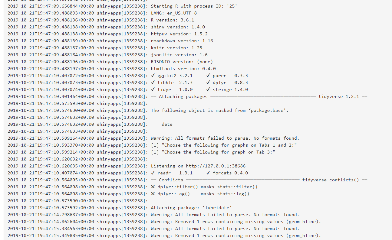
Thanks for the reply. I have included the the code now. Also tried checked the logs (see attached)

Is the problem with lubridate or the geom_hline?

The log suggest lubridate::ymd() is failing to parse the dates, maybe because your ERAS.rda file is not been read correctly. Could you share a sample of this file so we can take a look?

Hi, I've used dput() to show the below:

structure(list(ï..new_ID = c(589L, 581L, 490L, 489L, 488L, 487L, 
486L, 485L, 483L, 484L), ID = structure(1:10, .Label = c("1", 
"10", "100", "101", "102", "103", "104", "105", "106", "107", 
"108", "109", "11", "110", "111", "112", "113", "114", "115", 
"116", "117", "118", "119", "12", "120", "121", "122", "123", 
"124", "125", "126", "127", "128", "129", "13", "130", "131", 
"132", "133", "134", "135", "136", "137", "138", "139", "14", 
"140", "141", "142", "143", "144", "145", "146", "147", "148", 
"149", "15", "150", "151", "152", "153", "154", "155", "156", 
"157", "158", "159", "16", "160", "161", "162", "163", "164", 
"165", "166", "167", "168", "169", "17", "170", "171", "172", 
"173", "174", "175", "176", "177", "178", "179", "18", "180", 
"181", "182", "183", "184", "185", "186", "187", "188", "189", 
"19", "190", "191", "192", "193", "194", "195", "196", "197", 
"198", "199", "2", "20", "200", "201", "202", "203", "204", "205", 
"206", "207", "208", "209", "21", "210", "211", "212", "213", 
"214", "215", "216", "217", "218", "219", "22", "220", "221", 
"222", "223", "224", "225", "226", "227", "228", "229", "23", 
"230", "231", "232", "233", "234", "235", "236", "237", "238", 
"239", "24", "240", "241", "242", "243", "244", "245", "246", 
"247", "248", "249", "25", "250", "251", "252", "253", "254", 
"255", "256", "257", "258", "259", "26", "260", "261", "262", 
"263", "264", "265", "266", "267", "268", "269", "27", "270", 
"271", "272", "273", "274", "275", "276", "277", "278", "279", 
"28", "280", "281", "282", "283", "284", "285", "286", "287", 
"288", "289", "29", "290", "291", "292", "293", "294", "295", 
"296", "297", "298", "299", "3", "30", "300", "301", "302", "303", 
"304", "305", "306", "307", "308", "309", "31", "310", "311", 
"312", "313", "314", "315", "316", "317", "318", "319", "32", 
"320", "321", "322", "323", "324", "325", "326", "327", "328", 
"329", "33", "330", "331", "332", "333", "334", "335", "336", 
"337", "338", "339", "34", "340", "341", "342", "343", "344", 
"345", "346", "347", "348", "349", "35", "350", "351", "352", 
"353", "354", "355", "356", "357", "358", "359", "36", "360", 
"361", "362", "363", "364", "365", "366", "367", "368", "369", 
"37", "370", "371", "372", "373", "374", "375", "376", "377", 
"378", "379", "38", "380", "381", "382", "383", "384", "385", 
"386", "387", "388", "389", "39", "390", "391", "392", "393", 
"394", "395", "396", "397", "398", "399", "4", "40", "400", "401", 
"402", "403", "404", "405", "406", "407", "408", "409", "41", 
"410", "411", "412", "413", "414", "415", "416", "417", "418", 
"419", "42", "420", "421", "422", "423", "424", "425", "426", 
"427", "428", "429", "43", "430", "431", "432", "433", "434", 
"435", "436", "437", "438", "439", "44", "440", "441", "442", 
"443", "444", "445", "446", "447", "448", "449", "45", "450", 
"451", "452", "453", "454", "455", "456", "457", "458", "459", 
"46", "460", "461", "462", "463", "464", "465", "466", "467", 
"468", "469", "47", "470", "471", "472", "473", "474", "475", 
"476", "477", "478", "479", "48", "480", "481", "482", "483", 
"484", "485", "486", "487", "488", "489", "49", "490", "491", 
"492", "493", "494", "495", "496", "497", "498", "499", "5", 
"50", "500", "501", "502", "503", "504", "505", "506", "507", 
"508", "509", "51", "510", "511", "512", "513", "514", "515", 
"516", "517", "518", "519", "52", "520", "521", "522", "523", 
"524", "525", "526", "527", "528", "529", "53", "530", "531", 
"532", "533", "534", "535", "536", "537", "538", "539", "54", 
"540", "541", "542", "543", "544", "545", "546", "547", "548", 
"549", "55", "550", "551", "552", "553", "554", "555", "556", 
"557", "558", "559", "56", "560", "561", "562", "563", "564", 
"565", "566", "567", "568", "569", "57", "570", "571", "572", 
"573", "574", "575", "576", "577", "578", "579", "58", "580", 
"581", "582", "583", "584", "585", "586", "587", "588", "589", 
"59", "6", "60", "61", "62", "63", "64", "65", "66", "67", "68", 
"69", "7", "70", "71", "72", "73", "74", "75", "76", "77", "78", 
"79", "8", "80", "81", "82", "83", "84", "85", "86", "87", "88", 
"89", "9", "90", "91", "92", "93", "94", "95", "96", "97", "98", 
"99", "N1", "N2", "N3", "N4", "N5", "N6", "N7"), class = "factor"), 
    ASA = structure(c(2L, 2L, 2L, 2L, 3L, 1L, 2L, 2L, 3L, 2L), .Label = c("1", 
    "2", "3", "4"), class = "factor"), Weight = c(85, 71.05, 
    78, 71, 116.2, 87.3, 60, 57, 114, 112), BMI = c(36, 21, 27, 
    29, 34, 27, 24, 23, 41, 38), Preop_Hb = c(137L, 124L, 155L, 
    148L, 106L, 133L, 142L, 160L, 111L, 139L), Preop_MCV = c(94.4, 
    106.7, 96.4, 87.7, 75.3, 84, 79.6, 92.5, 77.6, 91.7), Anaemia = c(FALSE, 
    FALSE, FALSE, FALSE, TRUE, FALSE, FALSE, FALSE, TRUE, FALSE
    ), Postop_Hb = c(78, 102, 103, 131, 108, 109, 102, 128, 92, 
    114), BTS = structure(c(1L, 1L, 1L, 1L, 1L, 1L, 1L, 1L, 1L, 
    1L), .Label = c("No", "RCC"), class = "factor"), Units_BTS = c(0L, 
    0L, 0L, 0L, 0L, 0L, 0L, 0L, 0L, 0L), ACEI_ARB = c(FALSE, 
    FALSE, FALSE, TRUE, TRUE, FALSE, TRUE, FALSE, FALSE, FALSE
    ), Preop_Creat = c(62L, 52L, 96L, 52L, 52L, 59L, 50L, 82L, 
    56L, 68L), Pre_opGFR = c(60, 60, 60, 60, 60, 60, 60, 60, 
    60, 60), CKD = c("Nil", "Nil", "Nil", "Nil", "Nil", "Nil", 
    "Nil", "Nil", "Nil", "Nil"), AKI = structure(c(2L, 1L, 2L, 
    1L, 2L, 2L, 1L, 1L, 1L, 1L), .Label = c("0", "1", "2"), class = "factor"), 
    Postop_creat = c(NA, NA, NA, NA, NA, NA, NA, NA, NA, NA), 
    PreopOFe = c(0L, 0L, 0L, 0L, 1L, 0L, 0L, 0L, 0L, 1L), PostopOFe = c(NA, 
    NA, NA, NA, NA, NA, NA, NA, NA, NA), Pathology = structure(c(1L, 
    2L, 2L, 1L, 2L, 1L, 2L, 1L, 1L, 2L), .Label = c("Benign", 
    "Malignant"), class = "factor"), Sx_Approach = structure(c(2L, 
    1L, 1L, 1L, 2L, 1L, 1L, 1L, 1L, 3L), .Label = c("Laparoscopic", 
    "Lap-assisted", "Converted to open", "Open"), class = "factor"), 
    New_Stoma = structure(c(1L, 1L, 1L, 1L, 2L, 2L, 1L, 1L, 1L, 
    1L), .Label = c("N", "Y"), class = "factor"), DoA = structure(c(1563750000, 
    1561590000, 1548720000, 1548633600, 1548288000, 1548201600, 
    1548115200, 1548028800, 1547683200, 1547683200), class = c("POSIXct", 
    "POSIXt"), tzone = ""), DoS = structure(c(1563750000, 1561590000, 
    1548720000, 1548633600, 1548288000, 1548201600, 1548115200, 
    1548028800, 1547683200, 1547683200), class = c("POSIXct", 
    "POSIXt"), tzone = ""), Total_Time = c(295L, 276L, 289L, 
    478L, 380L, 540L, 264L, 201L, 290L, 240L), Intraop_Opioid = structure(c(1L, 
    1L, 4L, 1L, 2L, 4L, 4L, 1L, 2L, 4L), .Label = c("Both", "IV", 
    "Neither", "Spinal"), class = "factor"), LA_Use = c("IV Lidocaine & Spinal", 
    "IV Lidocaine & Spinal", "IV Lidocaine & Spinal", "IV Lidocaine & Spinal", 
    NA, "IV Lidocaine & Spinal", "IV Lidocaine & Spinal", "IV Lidocaine & Spinal", 
    NA, "IV Lidocaine & Spinal"), IVFluids_Stopped_D1 = structure(c(2L, 
    2L, 2L, 2L, 2L, 1L, 2L, 2L, 2L, 2L), .Label = c("N", "Y"), class = "factor"), 
    IVFluids_Restarted = structure(c(1L, 1L, 1L, 1L, 2L, 1L, 
    1L, 1L, 1L, 1L), .Label = c("N", "Y"), class = "factor"), 
    Mobilised_D1 = structure(c(2L, 2L, 2L, 1L, 2L, 2L, 1L, 2L, 
    1L, 2L), .Label = c("N", "Y"), class = "factor"), Diet_D1 = structure(c(2L, 
    2L, 2L, 2L, 2L, 2L, 2L, 2L, 2L, 2L), .Label = c("N", "Y"), class = "factor"), 
    Catheter_rm_D1 = structure(c(2L, 2L, 2L, 1L, 1L, 2L, 2L, 
    2L, 1L, 2L), .Label = c("N", "Y"), class = "factor"), Fluid_Volume = c(2791L, 
    3310L, 3891L, 2630L, 4451L, 3030L, 3180L, 2500L, 4280L, 4566L
    ), EBL = c(0, 500, 0, 300, 500, 200, 0, 0, 200, 0), DoDCC_met = structure(c(1564095600, 
    1561935600, 1548979200, 1548979200, 1548979200, 1548892800, 
    1548720000, 1548288000, 1548115200, 1548374400), class = c("POSIXct", 
    "POSIXt"), tzone = ""), DoDC = structure(c(1564095600, 1561935600, 
    1548979200, 1548979200, 1548979200, 1548892800, 1548720000, 
    1548288000, 1548115200, 1548374400), class = c("POSIXct", 
    "POSIXt"), tzone = ""), Delay_Reason = structure(c(NA_integer_, 
    NA_integer_, NA_integer_, NA_integer_, NA_integer_, NA_integer_, 
    NA_integer_, NA_integer_, NA_integer_, NA_integer_), .Label = c("Other", 
    "Other clinical", "Patient unwilling to be discharged", "Social"
    ), class = "factor"), Reoperation_Leak = structure(c(1L, 
    1L, 1L, 1L, 1L, 1L, 1L, 1L, 1L, 1L), .Label = c("N", "Y"), class = "factor"), 
    Reoperation_Other = structure(c(1L, 1L, 1L, 1L, 1L, 1L, 1L, 
    1L, 1L, 1L), .Label = c("N", "Y"), class = "factor"), ICU_Admission = structure(c(1L, 
    1L, 1L, 1L, 1L, 1L, 1L, 1L, 1L, 1L), .Label = c("N", "Y"), class = "factor"), 
    Readmission_30D = structure(c(1L, 1L, 1L, 1L, 1L, 2L, 1L, 
    1L, 1L, 1L), .Label = c("N", "Y"), class = "factor"), Readmission_spec = structure(c(NA, 
    NA, NA, NA, NA, 2L, NA, NA, NA, NA), .Label = c("Different", 
    "Same"), class = "factor"), Death_90D = structure(c(NA, 1L, 
    1L, 1L, 1L, 1L, 1L, 1L, 1L, 1L), .Label = c("N", "Y"), class = "factor"), 
    POMS_D3 = c(0L, 0L, 0L, 0L, 1L, 0L, 1L, 0L, 0L, 0L), POMS_D5 = c(0L, 
    0L, 0L, 0L, 0L, 1L, 1L, 0L, 0L, 1L), SORT = c(0.19, 0.37, 
    0.79, 0.41, 3.17, 0.19, 0.79, 0.19, 0.77, 0.37), Delayed_DC = structure(c(1L, 
    1L, 1L, 1L, 1L, 1L, 1L, 1L, 1L, 1L), .Label = c("N", "Y"), class = "factor"), 
    Preop_LOS = c(0L, 0L, 0L, 0L, 0L, 0L, 0L, 0L, 0L, 0L), Postop_LOS = c(4L, 
    4L, 3L, 4L, 8L, 8L, 7L, 3L, 5L, 8L), HDU_LOS = c(1L, 1L, 
    3L, 1L, 1L, 5L, 1L, 1L, 1L, 1L), Total_LOS = c(4L, 4L, 3L, 
    4L, 8L, 8L, 7L, 3L, 5L, 8L), Comments = structure(c(NA, NA, 
    NA, NA, 36L, NA, NA, NA, 36L, NA), .Label = c("#NAME?", "ADMITTED EARLIER - ALCOHOLIC", 
    "ADMITTEDTO ADMISSIONS DUE TO TARGET", "and appendicectomy + washout of pelvic abscess", 
    "and appendicectomy.", "and bilateral ureteric stents, TAH + BSO.", 
    "and bladder repair. ", "and BSO + TAH + ureteric stents ", 
    "and closure of ileostomy", "and defuctioning ileostomy", 
    "and defunctioning loop ileostomy", "and formation of end ileostomy", 
    "and ileostomy", "and left salpingectomy.", "and loop ileostomy", 
    "and repair of parastomal hernia", "and repair of parastomal hernia + end colostomy", 
    "and restorative ileo-anal pouch + defunctioning ileostomy", 
    "and right oopherectomy", "and small bowel resecton.  Waited for I+D axilla abscess", 
    "and TAH, BSO + ureteric stents.", "and TAH,BSO, SB resection x 2", 
    "and uretric stents + partial cystectomy + appendicectomy", 
    "AWI in situ/referred to OT", "CATHETER REMOVED 13.00", "catheter removed 18.00", 
    "catheter removed afternoon", "closure of sigmoid and duodenal fistulas also", 
    "confusion pod 3 AWI in situ", "copd and investigations for dementia", 
    "Due to bad weather", "fractured hip on admission", "hernia causing obstruction ", 
    "including prev ileo colonic anastomosis", "infected haematoma - surgery", 
    "No local anaesthetic given ", "patient died ", "patient refused to have catheter removed", 
    "readmission due to chemotherapy toxicity", "recatheterised", 
    "with closure of ileostomy + formation of colostomy"), class = "factor"), 
    Fluid_Balance = c(2791, 2810, 3891, 2330, 3951, 2830, 3180, 
    2500, 4080, 4566), Fluid_kg = c(32.8352941176471, 39.5496129486277, 
    49.8846153846154, 32.8169014084507, 34.0017211703959, 32.4169530355097, 
    53, 43.859649122807, 35.7894736842105, 40.7678571428571), 
    Risk = structure(c(1L, 1L, 1L, 1L, 2L, 1L, 1L, 1L, 1L, 1L
    ), .Label = c("Low", "Intermediate", "High", "Very High"), class = "factor"), 
    Obesity = structure(c(4L, 2L, 2L, 2L, 3L, 2L, 2L, 2L, 5L, 
    4L), .Label = c("Under", "Normal", "Obese", "Severe", "Morbid", 
    "Super"), class = "factor"), posPOMS3 = c(FALSE, FALSE, FALSE, 
    FALSE, TRUE, FALSE, TRUE, FALSE, FALSE, FALSE), posPOMS5 = c(FALSE, 
    FALSE, FALSE, FALSE, FALSE, TRUE, TRUE, FALSE, FALSE, TRUE
    ), Any_Two = c(FALSE, FALSE, FALSE, FALSE, TRUE, FALSE, TRUE, 
    FALSE, FALSE, FALSE), All_3 = c(TRUE, TRUE, TRUE, FALSE, 
    FALSE, TRUE, FALSE, TRUE, FALSE, TRUE), Weekday = structure(c(1L, 
    4L, 2L, 1L, 4L, 3L, 2L, 1L, 4L, 4L), .Label = c("Monday", 
    "Tuesday", "Wednesday", "Thursday", "Friday", "Saturday", 
    "Sunday"), class = "factor"), year_m = structure(c(1561935600, 
    1559343600, 1546300800, 1546300800, 1546300800, 1546300800, 
    1546300800, 1546300800, 1546300800, 1546300800), class = c("POSIXct", 
    "POSIXt"), tzone = ""), AKI_pos = c(TRUE, FALSE, TRUE, FALSE, 
    TRUE, TRUE, FALSE, FALSE, FALSE, FALSE)), row.names = c(NA, 
10L), class = "data.frame")

Please let me know if this is not suitable. As I mentioned, still very new to this.

In your sample data year_m column is of "POSIXct" class that is why ymd() is failing, see this example

lubridate::ymd(df$year_m)
#> Warning: All formats failed to parse. No formats found.
#>  [1] NA NA NA NA NA NA NA NA NA NA
lubridate::ymd_hms(df$year_m)
#>  [1] "2019-06-30 23:00:00 UTC" "2019-05-31 23:00:00 UTC"
#>  [3] "2019-01-01 00:00:00 UTC" "2019-01-01 00:00:00 UTC"
#>  [5] "2019-01-01 00:00:00 UTC" "2019-01-01 00:00:00 UTC"
#>  [7] "2019-01-01 00:00:00 UTC" "2019-01-01 00:00:00 UTC"
#>  [9] "2019-01-01 00:00:00 UTC" "2019-01-01 00:00:00 UTC"

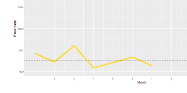
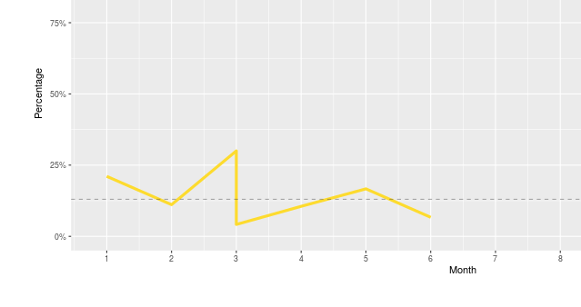
Thanks. I've done a workaround without using lubridate by using substr(). It has uploaded to server successfully and now I see the graph behaving strangely on the server compared to on my laptop:

How the graph is meant to look:
new_app

...How the graph looks on server:

server

I have now opened a new question as the problem is now off the original topic.

Thanks for your help on this @andresrcs

This topic was automatically closed 54 days after the last reply. New replies are no longer allowed.