Sample size calculation for two independent proportions

[QueryingQuagga]

Hello all
I have been trying to self-study different statistical concepts and have now found a use case that could be a relevant learning opportunity - calculating sample sizes for an experimental design.

Background

I have a marketing activity that I would like to test. The activity consists of an email campaign sent to a number of recipients with an intent to buy. What I'm recording is whether or not a recipient makes a purchase (purchase: yes / no).

In order to understand the effect of sending this email (that is, the proportion of recipients contacted that makes a purchase out of all recipients contacted - a conversion rate), I would like to hold out a group of customers who should not be contacted - a control group.

The question is: how many of my total group size should I (randomly) allocate to the control group?

I have some information from previous trials (note, these segments are independent - no one recipient is in both segment A and B):

| Year | Segment | Treatment (contacted) group size | Control (not contacted) group size | Conversion % for treatment | Conversion % for control |
|------|---------|----------------------------------|------------------------------------|----------------------------|--------------------------|
| 2022 | A       | 40000                            | 2000                               | 0.014 (1.4 %)              | 0.009 (0.9 %)            |
| 2022 | B       | 7000                             | 200                                | 0.007 (0.7 %)              | 0.0029 (0.29 %)          |

As I understand the design, in order to estimate the adequacy of this historical trial, I need to work with a two-sample test for proportions for unequal sample sizes.

I found the pwr package and tried testing the above historical studies by running the following code (assuming a significance level of 0.05 and a required power of 0.8):

# Seed
set.seed(42)

# libraries
library(pwr)

# Segment A
## Effect size
(effect_size_segment_A <- pwr::ES.h(p1 = 0.014, p2 = 0.009))
#> [1] 0.04717644

## Power calculation for two proportions (different sample sizes)
(pwr::pwr.2p2n.test(h = effect_size_segment_A, n1 = 40000, n2 = 2000, power = 0.8, sig.level = NULL, alternative = "two.sided"))
#> 
#>      difference of proportion power calculation for binomial distribution (arcsine transformation) 
#> 
#>               h = 0.04717644
#>              n1 = 40000
#>              n2 = 2000
#>       sig.level = 0.2227702
#>           power = 0.8
#>     alternative = two.sided
#> 
#> NOTE: different sample sizes

# Segment B
## Effect size
(effect_size_segment_B <- pwr::ES.h(p1 = 0.007, p2 = 0.0029))
#> [1] 0.05977242

## Power calculation for two proportions (different sample sizes)
(pwr::pwr.2p2n.test(h = effect_size_segment_B, n1 = 7000, n2 = 200, power = 0.8, sig.level = NULL, alternative = "two.sided"))
#> 
#>      difference of proportion power calculation for binomial distribution (arcsine transformation) 
#> 
#>               h = 0.05977242
#>              n1 = 7000
#>              n2 = 200
#>       sig.level = 0.7209852
#>           power = 0.8
#>     alternative = two.sided
#> 
#> NOTE: different sample sizes

^{Created on 2023-11-08 with reprex v2.0.2}

If my understanding and code is correct, it seems like the previous design for both trials were underpowered.

New trials

Now that I want to send out a new campaign activity, I have the chance of controlling the number of recipients that I should allocate to the control (or holdout) group. Below I have total segment size and effect size assumptions (in this case the assumed effect sizes are equal to those experienced in the previous trial):

| Year | Segment | Total segment size | Treatment (contacted) group size | Control (not contacted) group size | Assumed conversion % for treatment | Assumed conversion % for control |
|------|---------|--------------------|----------------------------------|------------------------------------|------------------------------------|----------------------------------|
| 2023 | A       | 60000              | ?                                | ?                                  | 0.014 (1.4 %)                      | 0.009 (0.9 %)                    |
| 2023 | B       | 4500               | ?                                | ?                                  | 0.007 (0.7 %)                      | 0.0029 (0.29 %)                  |

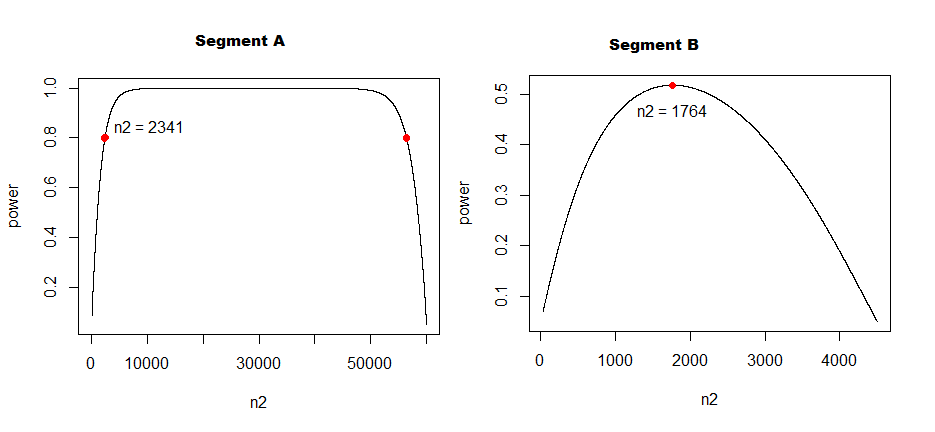
Following the logic from above, and assuming the same realised effect size as in the historical trial (the two proportions within each segment not falling any closer to each), I have ended up calculating the control group size like in the following:

# Seed
set.seed(42)

# libraries
library(pwr)

# Segment A
## Effect size
(effect_size_segment_A <- pwr::ES.h(p1 = 0.014, p2 = 0.009))
#> [1] 0.04717644

## Power calculation for two proportions (different sample sizes)
(pwr::pwr.2p2n.test(h = effect_size_segment_A, n1 = 56000, power = 0.8, sig.level = 0.05, alternative = "two.sided"))
#> 
#>      difference of proportion power calculation for binomial distribution (arcsine transformation) 
#> 
#>               h = 0.04717644
#>              n1 = 56000
#>              n2 = 3763.614
#>       sig.level = 0.05
#>           power = 0.8
#>     alternative = two.sided
#> 
#> NOTE: different sample sizes

# Segment B
## Effect size
(effect_size_segment_B <- pwr::ES.h(p1 = 0.007, p2 = 0.0029))
#> [1] 0.05977242

(pwr::pwr.2p2n.test(h = effect_size_segment_B, n1 = 4500, power = 0.8, sig.level = 0.05, alternative = "two.sided"))
#> 
#>      difference of proportion power calculation for binomial distribution (arcsine transformation) 
#> 
#>               h = 0.05977242
#>              n1 = 4500
#>              n2 = 4292.393
#>       sig.level = 0.05
#>           power = 0.8
#>     alternative = two.sided
#> 
#> NOTE: different sample sizes

^{Created on 2023-11-08 with reprex v2.0.2}

The above results seem reasonable, although it is obvious that segment B total size is hopelessly small.

Now to my main question:

1. Is this the correct statistical approach? Should I instead work with a chi sq test and a 2 x 2 matrix of the counts - if so, I would very much appreciate some guidance.

Regards

[MetinBulus]

Hi @QueryingQuagga,

There are several methods available for determining the sample size with unequal allocation in the context of an experimental design. Nevertheless, it is generally advisable to avoid an uneven allocation unless there are compelling reasons. Below, I will use the R package {pwrss} (https://pwrss.shinyapps.io/index/) to demonstrate various approaches that can be used to answer your question:

1. Proportion Difference

Change the kappa argument below for an unbalanced allocation to treatment and control groups. kappa is defined as the ratio of n1 / n2.

## Segment A
pwrss.z.2props(p1 = 0.014, p2 = 0.009, power = 0.80
               kappa = 1)

#>  Approach: Normal Approximation 
#>  Difference between Two Proportions 
#>  (Independent Samples z Test) 
#>  H0: p1 = p2 
#>  HA: p1 != p2 
#>  ------------------------------ 
#>   Statistical power = 0.8 
#>   n1 = 7135 
#>   n2 = 7135 
#>  ------------------------------ 
#>  Alternative = “not equal” 
#>  Non-centrality parameter = 2.802 
#>  Type I error rate = 0.05 
#>  Type II error rate = 0.2 

## Segment B
pwrss.z.2props(p1 = 0.007, p2 = 0.0029, power = 0.80
               kappa = 1)

#>   Approach: Normal Approximation 
#>   Difference between Two Proportions 
#>   (Independent Samples z Test) 
#>   H0: p1 = p2 
#>   HA: p1 != p2 
#>   ------------------------------ 
#>    Statistical power = 0.8 
#>    n1 = 4596 
#>    n2 = 4596 
#>   ------------------------------ 
#>   Alternative = “not equal” 
#>   Non-centrality parameter = 2.802 
#>   Type I error rate = 0.05 
#>   Type II error rate = 0.2 

2. Logistic Regression

Change prob argument below for an unbalanced allocation to treatment and control groups. prob is defined as the sampling rate which is the ratio of n1 / (n1 + n2). Also note that n = n1 + n2.

## Segment A
pwrss.z.logreg(p0 = 0.009, p1 = 0.014, power = 0.80, 
               distribution = list(dist = "bernoulli", prob = 0.50))

#>   Logistic Regression Coefficient 
#>   (Large Sample Approx. Wald's z Test) 
#>   H0: beta1 = 0 
#>   HA: beta1 != 0 
#>   Distribution of X = ‘bernoulli’ 
#>   Method = DEMIDENKO(VC) 
#>   ------------------------------ 
#>    Statistical power = 0.8 
#>    n = 14333 
#>   ------------------------------ 
#>   Alternative = “not equal” 
#>   Non-centrality parameter = 2.785 
#>   Type I error rate = 0.05 
#>   Type II error rate = 0.2 

## Segment B
pwrss.z.logreg(p0 = 0.007, p1 =  0.0029, power = 0.80,
               distribution = list(dist = "bernoulli", prob = 0.50))

#>   Logistic Regression Coefficient 
#>   (Large Sample Approx. Wald's z Test) 
#>   H0: beta1 = 0 
#>   HA: beta1 != 0 
#>   Distribution of X = ‘bernoulli’ 
#>   Method = DEMIDENKO(VC) 
#>    ------------------------------ 
#>    Statistical power = 0.8 
#>    n = 9369 
#>    ------------------------------ 
#>   Alternative = “not equal” 
#>   Non-centrality parameter = -2.738 
#>   Type I error rate = 0.05 
#>   Type II error rate = 0.2 

3. Chi-square Test
Uncertain how to incorporate unequal allocation here. Included here as per your question, in case you choose to conduct a chi-square test.

## Segment A
## create 2 x 2 table of cell probabilities as
cell.probs <- rbind(c(0.009, 0.014),
                    c(1 - 0.009, 1 - 0.014))

colnames(cell.probs) <- c("Control", "Treatment")
rownames(cell.probs) <- c("Purchased (Yes)", "Purchased (No)")
cell.probs

#>                  Control Treatment
#>  Purchased (Yes)   0.009    0.014
#>  Purchased (No)    0.991    0.986

## find the total sample size
pwrss.chisq.gofit(p1 = cell.probs, power = 0.80)

#>  Pearson's Chi-square Goodness-of-fit Test 
#>  for Contingency Tables 
#>   ------------------------------ 
#>   Statistical power = 0.8 
#>   Total n = 14276 
#>   ------------------------------ 
#>  Degrees of freedom = 1 
#>  Non-centrality parameter = 7.849
#>  Type I error rate = 0.05 
#>  Type II error rate = 0.2 

## Segment B
## create 2 x 2 table of cell probabilities as
cell.probs <- rbind(c(0.007, 0.0029),
                    c(1 - 0.007, 1 - 0.0029))

colnames(cell.probs) <- c("Control", "Treatment")
rownames(cell.probs) <- c("Purchased (Yes)", "Purchased (No)")
cell.probs

#>                 Control Treatment
#> Purchased (Yes)   0.007    0.0029
#> Purchased (No)    0.993    0.9971

## find the total sample size
pwrss.chisq.gofit(p1 = cell.probs, power = 0.80)

#>  Pearson's Chi-square Goodness-of-fit Test 
#>  for Contingency Tables 
#>  ------------------------------ 
#>   Statistical power = 0.8 
#>   Total n = 9200 
#>  ------------------------------ 
#>  Degrees of freedom = 1 
#>  Non-centrality parameter = 7.849 
#>  Type I error rate = 0.05 
#>  Type II error rate = 0.2 

[QueryingQuagga]

Thank you very much for your thorough response (and the great link to your shiny app!).

My reason for choosing an unequal allocation is based on a view of risk / opportunity:

• On the one hand I want to hold out enough recipients in order to allow a valid design from which I can believe in the fact that the activity (sending emails) has a positive effect that cannot be attributed to chance (with my assumed differences in conversion rates / an assumed effect size).

• On the other hand, since I want to send to as many as I can (since I believe that my profit will be maximized by doing the activity, as opposed to not doing it), I want to limit how many I reserve for the control group.

So it is a balancing act between not leaving money on the table (missed sales) and still allowing for a design that proves the continued effectiveness of the marketing activities (there are different segments receiving offers).

In effect: if I know:

• N: the total segment size
• Power: I would want 0.8 as a minimum
• Significance level: 0.05 as a minimum
• The assumed proportion that will purchase (the conversion rate) in each of the two groups (group1 control / group2 treatment)
• The alternative hypotesis should be greater / one-sided (the underlying assumption being that contacting customers with offer emails never lowers the proportion of buyers)

Then I would like to know the optimal allocation of individuals between the control group and the treatment group.

[MetinBulus]

I believe I understood your question. While there might be better solutions, the approach below should provide you with some insights.
For Segment A you need 2341 in control group while 57659 in treatment group.
For Segment B you need 1764 in control group while 2736 in treatment group.

Optimal Design for Segment A

• Total sample size is fixed at 60000.
• Power is constrained at 80%.
• Find minimum number of control group participants (n2).

total <- 60000
n2.vec <- seq(30, total, 1)
power.vec <- rep(NA, length(n2.vec))
for(i in 1:length(n2.vec)) {
  kappa <- (total / n2.vec[i]) - 1
  power.vec[i] <- pwrss.z.2props(p1 = 0.014, p2 = 0.009, n2 = n2.vec[i],
                                 kappa = kappa, alternative = "greater",
                                 verbose = FALSE)$power
}

idx <- which(round(power.vec, 3) == 0.800)
power.80 <- power.vec[idx]
n2.opt <- n2.vec[idx]
n2.opt

plot(n2.vec, power.vec, type = "l", xlab = "n2", ylab = "power")
points(x =  n2.opt, y = power.80, col = "red", pch = 16)
text("n2 = 2341", x =  n2.opt[1] + 8000, y = power.80[1] + 0.05)

Optimal Design for Segment B

• Total sample size is fixed at 4500.
• Maximize power rate.
• Find optimal number of control group participants (n2).

total <- 4500
n2.vec <- seq(30, total, 1)
power.vec <- rep(NA, length(n2s))
for(i in 1:length(n2.vec)) {
  kappa <- (total / n2.vec[i]) - 1
  power.vec[i] <- pwrss.z.2props(p1 = 0.007, p2 = 0.0029, n2 = n2.vec[i],
                                 kappa = kappa, alternative = "greater",
                                 verbose = FALSE)$power
}

idx <- which(power.vec == max(power.vec))
power.max <- power.vec[idx]
n2.opt <- n2.vec[idx]
n2.opt

plot(n2.vec, power.vec, type = "l", xlab = "n2", ylab = "power")
points(x =  n2.opt, y = power.max, col = "red", pch = 16)
text("n2 = 1764", x =  n2.opt, y = power.max - 0.05)

Figures

[QueryingQuagga]

Once again - thank you for your thorough response.

I have been reading your code and running it in R (I believe there is a small typetypo for segment B n2s should be n2.vec).

I do have a hard time replicating your results though. I have created the following example script for the above Segment A (the fixed total of 60000):

library(pwr)
library(pwrss)
library(purrr)
library(dplyr)
library(tidyr)
library(ggplot2)

set.seed(42)

# The total sample size available (N)
N_total_segment_size <- 60000
step <- 2

# Create simulated data with n1 / n2 combinations (+/- 2 steps)
sim_data <- tibble::tibble(
  total = N_total_segment_size,
  n1 = seq(from = (N_total_segment_size - step), to = step, by = -1),
  n2 = seq(from = step, to = (N_total_segment_size - step), by = 1),
  kappa = (N_total_segment_size / n2) - 1
)

# Run three different power tests over the n1 / n2 values in sim_data
test_results <- sim_data |>
  mutate(test_2p2n_arcsin = map2(
    # pwr::pwr.2p2n.test (with arcsin tranformation)
    n1, n2, \(n1, n2) pwr.2p2n.test(h = ES.h(p1 = 0.014, p2 = 0.009),
                                    n1 = n1,
                                    n2 = n2,
                                    sig.level = 0.05,
                                    power = NULL,
                                    alternative = "greater")),
    
    # pwrss:pwrss::pwrss.z.2props (without arcsin transformation)
    test_pwrss_z_2props_no_arcsin = map2(
      n2, kappa, \(n2, kappa) pwrss.z.2props(p1 = 0.014, p2 = 0.009,
                                             n2 = n2,
                                             kappa = kappa,
                                             alpha = 0.05,
                                             arcsin.trans = FALSE,
                                             alternative = "greater",
                                             verbose = FALSE)),
    
    # pwrss:pwrss::pwrss.z.2props (with arcsin transformation)
    test_pwrss_z_2props_arcsin = map2(
      n2, kappa, \(n2, kappa) pwrss.z.2props(p1 = 0.014, p2 = 0.009,
                                             n2 = n2,
                                             kappa = kappa,
                                             alpha = 0.05,
                                             arcsin.trans = TRUE,
                                             alternative = "greater",
                                             verbose = FALSE))
    )

# Pick out the power estimate within list structure of each 
test_results_power <- test_results |> 
  mutate(test_2p2n_arcsin_power = purrr::map_dbl(test_2p2n_arcsin, 5),
         test_pwrss_z_2props_no_arcsin_power = purrr::map_dbl(test_pwrss_z_2props_no_arcsin, 4),
         test_pwrss_z_2props_arcsin_power = purrr::map_dbl(test_pwrss_z_2props_arcsin, 4)) |>
  select(n1, n2, kappa, test_2p2n_arcsin_power, test_pwrss_z_2props_no_arcsin_power, test_pwrss_z_2props_arcsin_power)

(annotation_tibble <- test_results_power |>
  pivot_longer(
    cols = test_2p2n_arcsin_power:test_pwrss_z_2props_arcsin_power,
    names_to = "test_function",
    values_to = "power") |>
  group_by(test_function) |>
  filter(power >= 0.8) |> 
  slice(which.min(power)) |> 
  mutate(power_min_target = 0.8))
#> # A tibble: 3 × 6
#> # Groups:   test_function [3]
#>      n1    n2   kappa test_function                       power power_min_target
#>   <dbl> <dbl>   <dbl> <chr>                               <dbl>            <dbl>
#> 1 57079  2921 19.5    test_2p2n_arcsin_power              0.800              0.8
#> 2 57079  2921 19.5    test_pwrss_z_2props_arcsin_power    0.800              0.8
#> 3  3553 56447  0.0629 test_pwrss_z_2props_no_arcsin_power 0.800              0.8

result_long <- test_results_power |>
  pivot_longer(
    cols = test_2p2n_arcsin_power:test_pwrss_z_2props_arcsin_power,
    names_to = "test_function",
    values_to = "power")

result_long |> 
  ggplot(aes(x = n1, y = power)) +
  geom_line(linewidth = 1) +
  geom_hline(
    data = annotation_tibble,
    aes(yintercept = power_min_target)) +
  geom_point(
    data = annotation_tibble,
    mapping = aes(x = n1, y = power),
    size = 5,
    colour = "red") +
  geom_point(
    data = annotation_tibble,
    mapping = aes(x = n2, y = power),
    size = 5,
    colour = "red") +
  geom_label(
    data = annotation_tibble,
    aes(x = n1, y = power, label = n1),
    nudge_y = -0.025) +
  geom_label(
    data = annotation_tibble,
    aes(x = n2, y = power, label = n2),
    nudge_y = -0.025) +
  scale_y_continuous(
    n.breaks = 10,
    labels = scales::number_format(accuracy = 0.01, decimal.mark = "."),
    limits = c(0, 1.0)) +
  theme(legend.position = "none") +
  facet_wrap(~test_function)

^{Created on 2023-12-14 with reprex v2.0.2}

My main questions are:

1. Do you understand why there is such a difference in the control / treatment split of sample units?
2. What role does the arcsin transformation play in all of this? Do you know of any guidance in terms of what to choose and is a choice between the two dependent on sample size and or effect sizes?

Note, I'm unsure if the above has a small error - the treatment group point for test_pwrss_z_2props_no_arcsin_power is not aligning with the intercept for power = 0.8 and the power curve (the results seem correct when looking at the power test outputs and I believe the error might only be in the way I handle ggplot2)

[MetinBulus]

Hi @QueryingQuagga , your results are correct.

The arcsine transformation plays a crucial role in stabilizing the variance of the proportion difference. Consequently, it ensures a symmetric power function, yielding consistent kappa values on both the left and right. Results will be the same for different proportions that yield the same Cohen's h.

In contrast, the absence of the arcsine transformation results in an asymmetric power function, leading to disparate kappa values on the left and right. Results will diverge for different proportions that yield the same Cohen's h.

Probably you would want to use arcsine transformation for proportions towards extreme (0 and 1). Both approaches require large sample size for consistent estimates though. Essentially they are both z tests.

Here is a compact version of the code:

> library(pwrss)
> library(pwr)
> 
> # function for package {pwrss}
> opt.n2.pwrss <- function(x, total = 60000, target.power = 0.80, arcsin = TRUE) {
+     calc.power <- pwrss.z.2props(p1 = 0.014, p2 = 0.009, n2 = x,
+                                  kappa = (total / x) - 1, 
+                                  arcsin = arcsin,
+                                  alternative = "greater",
+                                  verbose = FALSE)$power
+   return(calc.power - target.power)
+ }
> 
> # function for package {pwr}
> opt.n2.pwr <- function(x, total = 60000, target.power = 0.80) {
+   calc.power <- pwr.2p2n.test(h = ES.h(p1 = 0.014, p2 = 0.009),
+                                 n1 = total - x,
+                                 n2 = x,
+                                 sig.level = 0.05,
+                                 power = NULL,
+                                 alternative = "greater")$power
+   return(calc.power - target.power)
+ }
> 
> 
> # optimal solutions
> sol1 <- uniroot(opt.n2.pwrss, arcsin = TRUE, interval = c(2,30000))$root
> sol2 <- uniroot(opt.n2.pwrss, arcsin = TRUE, interval = c(30000, 59998))$root
> sol3 <- uniroot(opt.n2.pwr, interval = c(2,30000))$root
> sol4 <- uniroot(opt.n2.pwr, interval = c(30000, 59998))$root
> sol5 <- uniroot(opt.n2.pwrss, arcsin = FALSE, interval = c(2,30000))$root
> sol6 <- uniroot(opt.n2.pwrss, arcsin = FALSE, interval = c(30000, 59998))$root
> 
> # summarize results
> n2 <- ceiling(c(sol1, sol2, sol3, sol4, sol5, sol6))
> n1 <- 60000 - n2
> kappa <- round(n1 / n2, 3)
> data.frame(package = c("pwrss", "pwrss", "pwr", "pwr", "pwrss", "pwrss"),
+            arcsin = c(TRUE, TRUE, TRUE, TRUE, FALSE, FALSE),
+            n2 = n2, n1 = n1, kappa = kappa,
+            power = rep(0.80, 6))
  package arcsin    n2    n1  kappa power
1   pwrss   TRUE  2921 57079 19.541   0.8
2   pwrss   TRUE 57080  2920  0.051   0.8
3     pwr   TRUE  2921 57079 19.541   0.8
4     pwr   TRUE 57080  2920  0.051   0.8
5   pwrss  FALSE  2345 57655 24.586   0.8
6   pwrss  FALSE 56448  3552  0.063   0.8