Prediction intervals with tidymodels, best practices?

What is the best practice for producing prediction intervals (not confidence intervals) for predictions using tidymodels (would prefer genralizable approach or at least across more than just linear regression and use of simulation methods when appropriate).

I read through these: https://github.com/tidymodels/parsnip/search?q=prediction+intervals&type=issues -- but got a little lost as seemed like was rolled into parsnip::predict() but also doesn't seem to have full set of features disucssed by Alex Hayes
Max in initial discussion... I was unclear exactly if this exists somewhere or will exist in the future.

I'm also interested if there are any good tidy tutorials out there on prediction intervals already that use existing tools (e.g. that take advantage of rsample, broom, etc).

(Link to helpful blog that breaks down sources of noise for bootstrapping prediction intervals: https://saattrupdan.github.io/2020-03-01-bootstrap-prediction/ , but code examples are in python).

This question was posted previously on the R4DS Online Learning Community Slack channel: https://rfordatascience.slack.com/archives/C8JSHANJY/p1601014414012500
1 Like

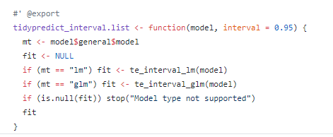
Have you looked at tidypredict?

2 Likes

Thanks for the reply and the link! I did check here but seemed to only be for parametric approach and also seemed to only be for linear models:

(Scrolling to bottom)
image

I would be interested in an example that uses simulation based approach as well as example for non-linear model.

parsnip can produce them for model types that naturally make them.

Otherwise... that paper that it cited in the blog post (and its references) are doable. I would not use the 632 method here since, for some models, the apparent error rate is 0. I would also use 10-fold CV to get the residuals too (instead of re-predicting the training set).

I have some old caret code laying around to do this (only for regression models). However, as the blog shows, you need to do a large number of bootstrap fits of the model to get good coverage and stability.

A long while back I tried this out at my previous job. There were some issues about the generality of the resampling approach. Imagine a CART tree fit. Outside of the data range, the predictions are flat on either side of the distribution of x and intervals can be really misleading there.

I've got a lot going on currently but I'll try to create a gist that does some of this with rsample and parsnip. I won't support it so use it at your own risk. I'll give a link here if/when I have that working.

6 Likes

Thank you!

parsnip can produce them for model types that naturally make them

I am assuming below is a way to check which parsnip supported models naturally make prediction intervals:

library(tidyverse)

envir <- parsnip::get_model_env()

ls(envir) %>% 
  tibble(name = .) %>% 
  filter(str_detect(name, "_predict")) %>% 
  mutate(prediction_modules  = map(name, parsnip::get_from_env)) %>% 
  unnest(prediction_modules) %>% 
  filter(str_detect(type, "pred_int"))
#> # A tibble: 3 x 5
#>   name                 engine mode           type     value           
#>   <chr>                <chr>  <chr>          <chr>    <list>          
#> 1 linear_reg_predict   lm     regression     pred_int <named list [4]>
#> 2 linear_reg_predict   stan   regression     pred_int <named list [4]>
#> 3 logistic_reg_predict stan   classification pred_int <named list [4]>

Created on 2020-09-29 by the reprex package (v0.3.0)

Code above is slightly modified from this github comment.

1 Like

Yes, that works fine.

I have managed to get a bootstrap working for logistic fits if you are interested.

1 Like

Yes, please share link.

The function fit_logistic in https://github.com/alankjackson/Covid/blob/master/app.R is where I do the bootstrap. Hopefully it will make sense. Take a look and let me know if you have questions. It's been a few months, but I remember it being relatively painful to get it working well. Making it robust against failure was the real challenge.

1 Like

I walked through fit_logistic() at your example. It looks like you are returning the bootstrapped confidence intervals, I am interested in the prediction intervals.

@Max
did you have reference related to below topic like paper

Outside of the data range, the predictions are flat on either side of the distribution of x and intervals can be really misleading there.

did you have reference for this topic

No; it's just the nature of that type of model. In 1D, it is a set of step functions.

@Max I got a little lost trying to work through the example in the paper / blog I'd shared :sweat_smile: (https://saattrupdan.github.io/2020-03-01-bootstrap-prediction/ ) and may have messed-up trying to encode it... :-/

  • I stuck with bootstrapping for the model variance component
  • Used cross validation for the variance in the residuals (per your suggestion) so skipped the whole adjustment around 632 and training/validation error

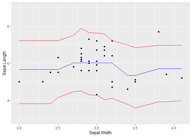
Here is a quick (attempted) example with decision trees and 90% prediction interval:

library(tidyverse)
library(tidymodels)

set.seed(123)

iris <- as_tibble(iris)
split <- initial_split(iris)

train <- training(split)
test <- testing(split)

model_variance <- rsample::bootstraps(train, sqrt(nrow(test))) %>%
  mutate(mod = map(splits, ~ rpart::rpart(Sepal.Length ~ Sepal.Width, data = analysis(.x))),
         test_preds = map(mod, ~ tibble(
           pred = predict(.x, test),
           index = seq_len(nrow(test))
         ))) %>%
  unnest(test_preds) %>%
  group_by(index) %>%
  mutate(m = pred - mean(pred)) %>%
  select(index, m, pred)

sampling_variance <- rsample::vfold_cv(train, 10) %>%
  mutate(
    mod = map(splits, ~ rpart::rpart(Sepal.Length ~ Sepal.Width, data = analysis(.x))),
    resids = map2(
      mod,
      splits,
      ~ predict(.x, assessment(.y)) - assessment(.y)$Sepal.Length
    )
  ) %>%
  select(resids) %>%
  unnest(resids) 

tidyr::crossing(model_variance, sampling_variance) %>% 
  mutate(c = m + resids + pred) %>% 
  group_by(index) %>% 
  summarise(q_05 = quantile(c, 0.05),
            q_95 = quantile(c, 0.95)) %>% 
  bind_cols(test, rpart::rpart(Sepal.Length ~ Sepal.Width, data = train) %>% predict(test) %>% tibble(.pred = .)) %>% 
  ggplot(aes(x = Sepal.Width))+
  geom_point(aes(y = Sepal.Length))+
  geom_line(aes(y = q_05), colour = "red")+
  geom_line(aes(y = q_95), colour = "red")+
  geom_line(aes(y = .pred), colour = "blue")+
  ylim(c(3, 9))

Created on 2021-02-12 by the reprex package (v0.3.0)

Could functionalize and edit so could take in a parsnip model specification and a recipe (but just wanted to get down a first attempt as wasn't sure if was doing correctly... :face_with_head_bandage:).

Other resources I found were this more simple approach:

Which essentially just uses randomized residuals (I imagine you would recommend using an alternative method for sampling the residuals here instead of pulling them from the model training/analysis set) -- not sure if this method may only be appropriate in linear models though...? Then there is the similar approach on Cross Validated which uses variance adjusted residuals (again assuming confined to linear models, and in this case relies on measure of influence).

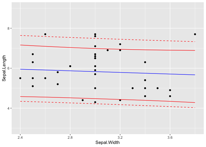
@brshallo I'm conflicted because, TBH, I'm not at all sold on this method. I definitely think that you need thousands of resamples to do this. I have some results below that show that the bands seem to be more narrow than the ones that we can compute analytically.

I do have some code for regression models but it's still not ready to be public. I'll try to put it in a gist soon.

Example:

library(tidyverse)
library(tidymodels)

set.seed(123)

iris <- as_tibble(iris)
split <- initial_split(iris)

train <- training(split)
test <- testing(split)

model_variance <- rsample::bootstraps(train, 5000) %>%
 mutate(mod = map(splits, ~ lm(Sepal.Length ~ Sepal.Width, data = analysis(.x))),
        test_preds = map(mod, ~ tibble(
         pred = predict(.x, test),
         index = seq_len(nrow(test))
        ))) %>%
 unnest(test_preds) %>%
 group_by(index) %>%
 mutate(m = pred - mean(pred)) %>%
 select(index, m, pred)

sampling_variance <- rsample::vfold_cv(train, 10) %>%
 mutate(
  mod = map(splits, ~ lm(Sepal.Length ~ Sepal.Width, data = analysis(.x))),
  resids = map2(
   mod,
   splits,
   ~ predict(.x, assessment(.y)) - assessment(.y)$Sepal.Length
  )
 ) %>%
 select(resids) %>%
 unnest(resids) 

lm_mod <- lm(Sepal.Length ~ Sepal.Width, data = iris)
analytical <- 
 predict(lm_mod, newdata = test, interval = "prediction") %>% 
 tibble::as_tibble() %>% 
 bind_cols(test)

tidyr::crossing(model_variance, sampling_variance) %>% 
 mutate(c = m + resids + pred) %>% 
 group_by(index) %>% 
 summarise(q_05 = quantile(c, 0.05),
           q_95 = quantile(c, 0.95)) %>% 
 bind_cols(test, lm(Sepal.Length ~ Sepal.Width, data = train) %>% predict(test) %>% tibble(.pred = .)) %>% 
 ggplot(aes(x = Sepal.Width))+
 geom_point(aes(y = Sepal.Length))+
 geom_line(aes(y = q_05), colour = "red")+
 geom_line(aes(y = q_95), colour = "red")+
 geom_line(aes(y = .pred), colour = "blue") + 
 geom_line(data = analytical, aes(y = lwr), col = "red", lty = 2) + 
 geom_line(data = analytical, aes(y = upr), col = "red", lty = 2) + 
 ylim(c(3, 9))

Created on 2021-02-12 by the reprex package (v1.0.0.9000)

1 Like

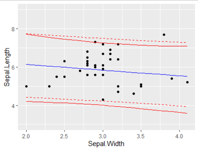
Interested to see what you put together! Also, just wanted to point out that some of the difference in your example is due to me using a 90% prediction interval rather than 95%, the default level for predict() (sorry for using a weird alpha :sweat_smile:).

If you change the quantile() arguments to 0.025 and 0.975 respectively, you'll get:
image

1 Like

Ah ok. My bad. Looks better

I put the above approach into a couple rough/quick functions: prep_interval() that is set-up to take in a workflow (with a recipe and model specification) and output a list containing objects needed to produce new prediction intervals and then predict_interval() that takes in the output from the above function + new data to produce prediction intervals on. See gist referenced below for documentation. The code below should essentially be equivalent to my prior example with rpart...

library(tidyverse)
library(tidymodels)

set.seed(123)

iris <- as_tibble(iris)
split <- initial_split(iris)

train <- training(split)
test <- testing(split)

dt_mod <- parsnip::decision_tree() %>% 
  set_engine("rpart") %>% 
  set_mode("regression")

dt_rec <- recipe(Sepal.Length ~ Sepal.Width, data = train)

dt_wf <- workflows::workflow() %>% 
  add_model(dt_mod) %>% 
  add_recipe(dt_rec)

devtools::source_gist("https://gist.github.com/brshallo/3db2cd25172899f91b196a90d5980690")

# Maybe would be better to allow a more custom resamples object as well...
prepped_for_interval <- prep_interval(dt_wf, train)

prepped_for_interval
#> $model_uncertainty
#> # A tibble: 10 x 2
#>    fit      recipe  
#>    <list>   <list>  
#>  1 <fit[+]> <recipe>
#>  2 <fit[+]> <recipe>
#>  3 <fit[+]> <recipe>
#>  4 <fit[+]> <recipe>
#>  5 <fit[+]> <recipe>
#>  6 <fit[+]> <recipe>
#>  7 <fit[+]> <recipe>
#>  8 <fit[+]> <recipe>
#>  9 <fit[+]> <recipe>
#> 10 <fit[+]> <recipe>
#> 
#> $sample_uncertainty
#> # A tibble: 113 x 1
#>     .resid
#>      <dbl>
#>  1  1.25  
#>  2 -0.0444
#>  3  0.256 
#>  4 -0.100 
#>  5  1.75  
#>  6  0.556 
#>  7 -0.543 
#>  8 -0.453 
#>  9  0.947 
#> 10 -0.443 
#> # ... with 103 more rows

pred_interval <- predict_interval(prepped_for_interval, test, probs = c(0.05, 0.95)) 

pred_interval
#> # A tibble: 37 x 2
#>    probs_0.05 probs_0.95
#>         <dbl>      <dbl>
#>  1       4.26       7.31
#>  2       4.00       7.02
#>  3       3.90       6.82
#>  4       4.40       7.69
#>  5       3.71       6.73
#>  6       4.00       7.01
#>  7       4.26       7.29
#>  8       3.70       6.74
#>  9       4.54       7.88
#> 10       3.91       7.26
#> # ... with 27 more rows

Created on 2021-03-04 by the reprex package (v0.3.0)

@Max the correct approach may be to lean on research in conformal prediction / inference. I pasted a few resources I skimmed below, though need to look into more closely (it seems like much of the research here comes out of either Carnegie Mellon or Royal Holloway University, London):

Resources suggest some methods may have high computation costs (e.g. jackknife+), others less so (e.g. split-conformal)... but again, need to read more closely.

1 Like

I am finishing up a 3-part series of posts on prediction intervals that has examples with {tidymodels}:

Below is a short {tidymodels} wishlist for support of prediction intervals (feel free to ignore, more just getting down my notes):

  • Broader support for quantiles, e.g. {quantreg} in {parsnip}, predict() method for type = "quantiles" per parsnip#119, ...
  • Measures for prediction intervals like "coverage" and "interval width" being added to {yardstick} or an extension package. OR guidance on custom metrics being edited so doesn't require an estimate argument (as would probably want arguments like truth, upper, lower ...)
  • Support for some kind of out-of-sample based method, e.g. something like the workflow %>% prep_interval(train_data) %>% predict_interval(new_data) I go through in Part 2a or support for conformal inference

@Max if you have an interest in me opening an issue pertaining to any of these or helping out in another way feel free to let me know.

1 Like

Obviously Max will be able to say whether or not implementation is likely, but would you mind posting GH issues for them, and maybe linking back to this post either way?

I'm just thinking it would be good to have your wishlist items in the respective package repos for discussion's sake/seeing them in the future. :slightly_smiling_face:

BTW, really cool posts! I'm reading them through now.