How to obtain prediction intervals from XGBoost regression made with tidymodels?

A simple, minimal XGBoost regression adapted from various tutorials by @julia :

library(tidymodels)
library(tidypredict)

tidymodels_prefer()

#Initial split, generate training and testing
mysplit <- initial_split(iris %>% select(-Species), strata=Petal.Width)
training_set <- training(mysplit)
test_set <- testing(mysplit)


#Set up the model specification
#The hyperparameters will be tuned
xgb_spec <- boost_tree(
    trees = 1000,
    tree_depth = tune(),
    min_n = tune(),
    loss_reduction = tune(),                    
    sample_size = tune(),
    mtry = tune(),   
    learn_rate = tune()                          
) %>%
    set_engine("xgboost") %>%
    set_mode("regression")


#Set up a space-filling grid design to cover the hyperparameter space as well as possible
xgb_grid <- grid_latin_hypercube(
    tree_depth(),
    min_n(),
    loss_reduction(),
    sample_size = sample_prop(),
    finalize(mtry(), training_set), #gets treated differently b/c it depends on actual # of predictors in data
    learn_rate(),
    size = 30
)

#Put the model specification into a workflow
xgb_wf <- workflow() %>%
    add_formula(Petal.Width ~.) %>% 
    add_model(xgb_spec)


#Create cross-validation resamples for tuning the model
input_folds <- vfold_cv(training_set, strata=Petal.Width)


#Use tunable workflow to tune
doParallel::registerDoParallel()
xgb_res <- tune_grid(
    xgb_wf,
    resamples = input_folds,
    grid = xgb_grid,
    control = control_grid(save_pred = TRUE)
)


#Select the best parameters based on RMSE
best_rmse <- select_best(xgb_res, "rmse")


#Finalize the tuneable workflow using the best parameters
final_xgb <- finalize_workflow(
    xgb_wf,
    best_rmse
)

#############
#Fit the final best model to training set and evaluate the test set
final_res <- last_fit(final_xgb, mysplit)
#############


#Get the model-predicted values of the test set
pred_df <- 
    final_res %>%
    collect_predictions() %>%
    as.data.frame()

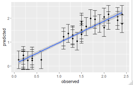
How can I obtain prediction intervals for the predictions? I want to get an idea for the uncertainty associated with each prediction, as in 95% prediction intervals.

I know that collect_metrics() will give me error estimates, but that is a general idea of model performance.

Prediction intervals have been previously discussed here with some interesting comments from @max and ultimately a fantastic blog post from @brshallo .

However - it's not clear if a Boostrap approach to prediction intervals could work for XGBoost regression, like here in my tuned model. Could I apply it such that I don't have to re-do the prediction and double the computation time? If so, how could I adapt the above code to produce the prediction intervals?

Thanks!

it's not clear if a Boostrap approach to prediction intervals could work for XGBoost regression, like here in my tuned model.

I think the bootstrap method is appropriate for almost any model, including boosted trees. They do take a while to compute, though.

Alternatively, the package probably has some tools for conformal inference that can give you prediction intervals for regression models (I'll implement them for classification after our conference).

I just published a tutorial on tidymodels.org about them. You'll need a decent amount of data to get good interval estimates (for some definition of "decent"), but they can be computed without bootstrapping.

2 Likes

@Max Thanks for this beautiful tutorial! I ran through it, and learned about techniques I was previously unaware of (and that i may need to beware of how boosted trees like my example react to some of them).

Could you tell me how to apply conformal inference to obtain the prediction intervals from my minimal reprex above? My 'real' data is large.

I really would like to know how to use this technique here and where....in my case final_xgb is the best workflow, and final_res is the result from applying final_xgb on the test set. ...so is it appropriate to obtain prediction intervals for output of final_res, and how do I do that with the probably package?

One attempt was problematic due to last_fit object not being compatible with int_conformal_split

Thanks!

This isn't the best data set for an example, but here you go...

(my additions shown with #Max)

library(tidymodels)
library(probably)
#> 
#> Attaching package: 'probably'
#> The following objects are masked from 'package:base':
#> 
#>     as.factor, as.ordered

tidymodels_prefer()

#Initial split, generate training and testing
mysplit <- initial_split(iris %>% select(-Species), strata = Petal.Width)
training_set <- training(mysplit)
test_set <- testing(mysplit)


#Set up the model specification
#The hyperparameters will be tuned
xgb_spec <- boost_tree(
  trees = 1000,
  tree_depth = tune(),
  min_n = tune(),
  loss_reduction = tune(),                    
  sample_size = tune(),
  mtry = tune(),   
  learn_rate = tune()                          
) %>%
  set_engine("xgboost") %>%
  set_mode("regression")


#Set up a space-filling grid design to cover the hyperparameter space as well as possible
xgb_grid <- grid_latin_hypercube(
  tree_depth(),
  min_n(),
  loss_reduction(),
  sample_size = sample_prop(),
  finalize(mtry(), training_set), #gets treated differently b/c it depends on actual # of predictors in data
  learn_rate(),
  size = 30
)

#Put the model specification into a workflow
xgb_wf <- workflow() %>%
  add_formula(Petal.Width ~.) %>% 
  add_model(xgb_spec)

# Max: set the seed for reproducability
set.seed(1)
#Create cross-validation resamples for tuning the model
input_folds <- vfold_cv(training_set, strata=Petal.Width)

# Max: set the seed for reproducability
set.seed(2)
xgb_res <- tune_grid(
  xgb_wf,
  resamples = input_folds,
  grid = xgb_grid,
  control = control_grid(save_pred = TRUE, extract = I)
)
#> → A | warning: A correlation computation is required, but `estimate` is constant and has 0 standard deviation, resulting in a divide by 0 error. `NA` will be returned.
#> There were issues with some computations   A: x1
#> There were issues with some computations   A: x2
#> There were issues with some computations   A: x3
#> There were issues with some computations   A: x4
#> There were issues with some computations   A: x5
#> There were issues with some computations   A: x6
#> There were issues with some computations   A: x7
#> There were issues with some computations   A: x8
#> There were issues with some computations   A: x9
#> There were issues with some computations   A: x10
#> 


#Select the best parameters based on RMSE
best_rmse <- select_best(xgb_res, "rmse")

# Max: create a conformal inference object
conf_cv_res <- int_conformal_cv(xgb_res, parameters = best_rmse)
conf_cv_res
#> Conformal inference via CV+
#> preprocessor: formula 
#> model: boost_tree (engine = xgboost) 
#> number of models: 10 
#> training set size: 110 
#> 
#> Use `predict(object, new_data, level)` to compute prediction intervals

#Finalize the tuneable workflow using the best parameters
final_xgb <- finalize_workflow(
  xgb_wf,
  best_rmse
)

#############
#Fit the final best model to training set and evaluate the test set
final_res <- last_fit(final_xgb, mysplit)

# Max: 
test_set_pred <- collect_predictions(final_res)
test_set_intervals <- predict(conf_cv_res, test_set)
# Note that there is also a .pred column here. That is the average of the 10
# predictions from cross-validation and is probably slightly different from
# what you get above. 
test_set_intervals
#> # A tibble: 40 × 3
#>    .pred_lower .pred .pred_upper
#>          <dbl> <dbl>       <dbl>
#>  1      -0.162 0.323       0.809
#>  2      -0.245 0.240       0.725
#>  3      -0.162 0.323       0.809
#>  4      -0.245 0.240       0.725
#>  5      -0.162 0.323       0.809
#>  6      -0.162 0.323       0.809
#>  7      -0.162 0.323       0.809
#>  8      -0.162 0.323       0.809
#>  9      -0.162 0.323       0.809
#> 10      -0.228 0.257       0.742
#> # ℹ 30 more rows

Created on 2023-08-17 with reprex v2.0.2

2 Likes

Thanks, I was able to apply this successfully! Just a couple quick follow-ups:

  1. Is this the 95% prediction interval? Can that be modified?

  2. The '.pred' values produced from predict(conf_cv_res, test_set) are indeed slightly different than '.pred' values from collect_predictions() , but just very slightly in my bigger example. If the predict() version is the average across the CVs, what was the original version producing? Any suggestion on which to trust more? (doesn't seem like either will be bad)

Thanks a ton!

EDIT: After some further digging I think it is 95% PIs and that can be clarified with test_set_intervals <- predict(conf_cv_res, test_set, level = 0.95)

Also I think it may be best to essentially disregard the .pred column obtained from the original method of collect_predictions(), and focus on the .pred column produced predict(conf_cv_res, test_set) along with their associated PIs.

That's what I would do.

1 Like

Uh oh... found something unexpected. The difference in prediction intervals (upper minus lower) is the same for every measurement. I don't think this should be the case.

Appending your example to calculate the difference between upper and lower preds, then plotting (modified at the end):

library(tidymodels)
library(probably)
#> 
#> Attaching package: 'probably'
#> The following objects are masked from 'package:base':
#> 
#>     as.factor, as.ordered

tidymodels_prefer()

#Initial split, generate training and testing
mysplit <- initial_split(iris %>% select(-Species), strata = Petal.Width)
training_set <- training(mysplit)
test_set <- testing(mysplit)


#Set up the model specification
#The hyperparameters will be tuned
xgb_spec <- boost_tree(
  trees = 1000,
  tree_depth = tune(),
  min_n = tune(),
  loss_reduction = tune(),                    
  sample_size = tune(),
  mtry = tune(),   
  learn_rate = tune()                          
) %>%
  set_engine("xgboost") %>%
  set_mode("regression")


#Set up a space-filling grid design to cover the hyperparameter space as well as possible
xgb_grid <- grid_latin_hypercube(
  tree_depth(),
  min_n(),
  loss_reduction(),
  sample_size = sample_prop(),
  finalize(mtry(), training_set), #gets treated differently b/c it depends on actual # of predictors in data
  learn_rate(),
  size = 30
)

#Put the model specification into a workflow
xgb_wf <- workflow() %>%
  add_formula(Petal.Width ~.) %>% 
  add_model(xgb_spec)

# Max: set the seed for reproducability
set.seed(1)
#Create cross-validation resamples for tuning the model
input_folds <- vfold_cv(training_set, strata=Petal.Width)

# Max: set the seed for reproducability
set.seed(2)
xgb_res <- tune_grid(
  xgb_wf,
  resamples = input_folds,
  grid = xgb_grid,
  control = control_grid(save_pred = TRUE, extract = I)
)
#> → A | warning: A correlation computation is required, but `estimate` is constant and has 0 standard deviation, resulting in a divide by 0 error. `NA` will be returned.
#> There were issues with some computations   A: x1
#> There were issues with some computations   A: x2
#> There were issues with some computations   A: x3
#> There were issues with some computations   A: x4
#> There were issues with some computations   A: x5
#> There were issues with some computations   A: x6
#> There were issues with some computations   A: x7
#> There were issues with some computations   A: x8
#> There were issues with some computations   A: x9
#> There were issues with some computations   A: x10
#> 


#Select the best parameters based on RMSE
best_rmse <- select_best(xgb_res, "rmse")

# Max: create a conformal inference object
conf_cv_res <- int_conformal_cv(xgb_res, parameters = best_rmse)
conf_cv_res
#> Conformal inference via CV+
#> preprocessor: formula 
#> model: boost_tree (engine = xgboost) 
#> number of models: 10 
#> training set size: 110 
#> 
#> Use `predict(object, new_data, level)` to compute prediction intervals

#Finalize the tuneable workflow using the best parameters
final_xgb <- finalize_workflow(
  xgb_wf,
  best_rmse
)

#############
#Fit the final best model to training set and evaluate the test set
final_res <- last_fit(final_xgb, mysplit)

# Max: 
test_set_pred <- collect_predictions(final_res)
test_set_intervals <- predict(conf_cv_res, test_set)
# Note that there is also a .pred column here. That is the average of the 10
# predictions from cross-validation and is probably slightly different from
# what you get above. 
test_set_intervals
#> # A tibble: 40 × 3
#>    .pred_lower .pred .pred_upper
#>          <dbl> <dbl>       <dbl>
#>  1      -0.162 0.323       0.809
#>  2      -0.245 0.240       0.725
#>  3      -0.162 0.323       0.809
#>  4      -0.245 0.240       0.725
#>  5      -0.162 0.323       0.809
#>  6      -0.162 0.323       0.809
#>  7      -0.162 0.323       0.809
#>  8      -0.162 0.323       0.809
#>  9      -0.162 0.323       0.809
#> 10      -0.228 0.257       0.742
#> # ℹ 30 more rows
#> 
#> 

#What is the difference in PI magnitude between each measurement/prediction?
test_set_intervals <- 
  test_set_intervals %>%
  mutate("pred_diff"=.pred_upper - .pred_lower) %>%
  mutate("obs_data"=test_set$Petal.Width) #Add in the observed test set data 

test_set_intervals %>%
  ggplot(aes(x=obs_data, y=.pred)) +
  geom_point() +
  geom_errorbar(aes(ymin = .pred_lower,
                    ymax = .pred_upper)) +
  xlab("observed") +
  ylab("predicted") +
  geom_smooth(method="lm")

The prediction intervals (shown as error bars here) are all the same size :
image

This isn't a perfect dataset, but I think you'd still expect points closer to the y=x line to have tighter/smaller Prediction Intervals. At the very least, they should not all be exactly the same size, no?

Thanks for your help @Max

(Edit) : Or is this just how conformal prediction works and I have to move to quantile regression or boostrapping (and re-training model multiple times) to get intervals of varying widths?

Most basic conformal intervals work this way (equal widths). You can use conformalized quantile regression to create adaptive width intervals (but note that they extrapolate very poorly). See ?int_conformal_quantile.

Thanks @Max! after reading up on this I think it's what might be best for my current needs. I'm trying to adapt the above minimal reprex to int_conformal_quantile but it seems like I keep either choosing the wrong object or am not setting up the cal_data properly. How can I adapt it to be used correctly with int_conformal_quantile to get the adaptive width intervals?

Thanks again.

This topic was automatically closed 7 days after the last reply. New replies are no longer allowed.

If you have a query related to it or one of the replies, start a new topic and refer back with a link.