Plot large data in R

Hi,

Asking help for plotting large data in R.

I have 10millions data, with different dataID.
I picked dataID=35, so there are 7567 records.

From that 7567records, I tried to plot the first 50data, using this

ggplot(PlotD, aes(x = localminute, y = meter_value)) + geom_point() + ggtitle("meter value for dataID=35") + theme(axis.text.x = element_text(angle = 90, hjust = 1))

the plot is perfect, just the x-axis (local minute) is not in chronological order. the x-axis is plotted in numerical order,

for example, the plotted x-axis is in this sequence:
1/10/2015 0:14
1/10/2015 0:42 jumped to
1/10/2015 11:24

image

First 50data, as below:
|localminute|dataid|meter_value|
|1/10/2015 0:14|35|93470|
|1/10/2015 0:42|35|93470|
|1/10/2015 2:02|35|93470|
|1/10/2015 2:12|35|93470|
|1/10/2015 2:20|35|93470|
|1/10/2015 2:23|35|93470|
|1/10/2015 3:59|35|93470|
|1/10/2015 4:30|35|93470|
|1/10/2015 4:34|35|93470|
|1/10/2015 5:14|35|93470|
|1/10/2015 5:17|35|93470|
|1/10/2015 6:23|35|93472|
|1/10/2015 7:26|35|93472|
|1/10/2015 8:19|35|93472|
|1/10/2015 8:44|35|93472|
|1/10/2015 8:54|35|93472|
|1/10/2015 9:36|35|93472|
|1/10/2015 11:24|35|93474|
|1/10/2015 12:29|35|93474|
|1/10/2015 15:04|35|93474|
|1/10/2015 15:20|35|93474|
|1/10/2015 16:22|35|93474|
|1/10/2015 17:03|35|93476|
|1/10/2015 17:11|35|93476|
|1/10/2015 17:24|35|93476|
|1/10/2015 17:54|35|93476|
|1/10/2015 18:02|35|93476|
|1/10/2015 18:59|35|93476|
|1/10/2015 19:44|35|93482|
|1/10/2015 19:57|35|93482|
|1/10/2015 21:13|35|93484|
|1/10/2015 21:16|35|93484|
|1/10/2015 21:33|35|93484|
|1/10/2015 21:54|35|93484|
|1/10/2015 22:34|35|93484|
|1/10/2015 23:07|35|93484|
|1/10/2015 23:57|35|93484|
|2/10/2015 0:01|35|93484|
|2/10/2015 1:14|35|93484|
|2/10/2015 1:24|35|93484|
|2/10/2015 2:15|35|93484|
|2/10/2015 3:35|35|93486|
|2/10/2015 3:50|35|93486|
|2/10/2015 4:24|35|93486|
|2/10/2015 5:44|35|93486|
|2/10/2015 6:13|35|93486|
|2/10/2015 6:17|35|93486|
|2/10/2015 7:07|35|93486|
|2/10/2015 8:53|35|93488|
|2/10/2015 9:05|35|93488|


For plotting all 7567 datas, using the same code
"ggplot(PlotD, aes(x = localminute, y = meter_value)) + geom_point() + ggtitle("meter value for dataID=35") + theme(axis.text.x = element_text(angle = 90, hjust = 1)) "

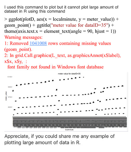
As output the plot is randomly scattered and i could not see the horizontal x-axis data label.

I got this Warning messages:
1: Removed 1041008 rows containing missing values (geom_point).
2: In grid.Call.graphics(L_text, as.graphicsAnnot(x$label), x$x, x$y, :
font family not found in Windows font database

1 Like

Based on the error message, it sounds like you're missing quite a bit of data (perhaps consider filtering before plotting), and you're also missing the base font family.

Could you please turn this into a self-contained reprex (short for minimal reproducible example)? It will help us help you if we can be sure we're all working with/looking at the same stuff.

Right now the best way to install reprex is:

# install.packages("devtools")
devtools::install_github("tidyverse/reprex")

If you've never heard of a reprex before, you might want to start by reading the tidyverse.org help page. The reprex dos and don'ts are also useful.

If you run into problems with access to your clipboard, you can specify an outfile for the reprex, and then copy and paste the contents into the forum.

reprex::reprex(input = "fruits_stringdist.R", outfile = "fruits_stringdist.md")

For pointers specific to the community site, check out the reprex FAQ, linked to below.

1 Like

Hi, what happens if you only run the first geom: ggplot(plotD, aes(x = localminute, y = meter_value)) + geom_point()?

Hi all,

Thanks alot for your each replies, I will try what you suggested. I just started learning R language, for data analysing

I used Microsoft visual studio 2017, R
Currently using R interactive windows to test the R-codes.

I uploaded the output of the graph for plotting 7567 filtered data, from the graph, I could not see the X-axis data label and the data plotting also seems not correct!

Appreciate for your help :slight_smile:

I am guessing from the error message that the "plotD" data frame has over 1M rows that are missing valid values for localminute and/or meter_value. So it might not be filtered in the way you intended.

I'm also guessing from the x axis of your chart that your localminute column might be formatted as a character field and not as a date-time. That might explain the strange periodicity of your chart, if ggplot is simply sorting your time stamps in alphabetical, not chronological, order. If this is the case, and assuming you have installed the "tidyverse" package, you could write the following to convert the localminute data, and then re-run your plot.

plotD <- 
  plotD %>%
  mutate(localminute = lubridate::mdy_hm(localminute)

By the way, the mdy_hm function assumes your data is in order of "month, day, year, hour, minute." It's ambiguous from your data if you actually meant it to be interpreted as being in "day, month, year, hour, minute" order. If that's what your data means, you'd use the "dmy_hm" function...

3 Likes

Hi jonspring

I tried what u suggested,

PlotD <- PlotD %>% mutate(localminute = lubridate::dmy_hms(localminute))
Warning message:
All formats failed to parse. No formats found.

Hi Mara,

Is it okay, if I didnt use the reprex? I just roughly go through the link, you provided but I still lost..

Basically, how does that reprex will help for data analyzing using R?

This thread had couple of good suggestions for plotting large data which could be beneficial for your case

The point of a reprex is to give the community a way to reproduce the same problem you're having. That way they can investigate and test various potential solutions so they can provide you the most useful one.

In your case, it looked to me like there's something not working with your x axis that is preventing ggplot from interpreting the data chronologically in order of localminute. That would explain the strange periodicity of your chart, which looks like it might be a single ascending series, but currently shown out of order.

You went through the trouble of pasting some example data which confirms my suspicion that ggplot is interpreting your time stamps as text, and shows that your data is in day-month-year order. A reprex would go the next step of letting people who want to help you to load that exact data, play with it, and check whether a given solution works. Without a reprex, we sometimes have to "play chess by mail" as you try out each of the suggestions people send you.

For next time, I would suggest including the data in a way people can load it directly. I created the data below using your edited question's data and the addin here. Then other R users can work with a copy of exactly what you're using.

library(tidyverse)


PlotD <- 
  tibble::tribble(
  ~localminute, ~dataid, ~meter_value,
    "1/10/2015 0:14",     35L,       93470L, 
    "1/10/2015 0:42",     35L,       93470L, 
    "1/10/2015 2:02",     35L,       93470L, 
    "1/10/2015 2:12",     35L,       93470L, 
    "1/10/2015 2:20",     35L,       93470L, 
    "1/10/2015 2:23",     35L,       93470L, 
    "1/10/2015 3:59",     35L,       93470L, 
    "1/10/2015 4:30",     35L,       93470L, 
    "1/10/2015 4:34",     35L,       93470L, 
    "1/10/2015 5:14",     35L,       93470L, 
    "1/10/2015 5:17",     35L,       93470L, 
    "1/10/2015 6:23",     35L,       93472L, 
    "1/10/2015 7:26",     35L,       93472L, 
    "1/10/2015 8:19",     35L,       93472L, 
    "1/10/2015 8:44",     35L,       93472L, 
    "1/10/2015 8:54",     35L,       93472L, 
    "1/10/2015 9:36",     35L,       93472L, 
   "1/10/2015 11:24",     35L,       93474L, 
   "1/10/2015 12:29",     35L,       93474L, 
   "1/10/2015 15:04",     35L,       93474L, 
   "1/10/2015 15:20",     35L,       93474L, 
   "1/10/2015 16:22",     35L,       93474L, 
   "1/10/2015 17:03",     35L,       93476L, 
   "1/10/2015 17:11",     35L,       93476L, 
   "1/10/2015 17:24",     35L,       93476L, 
   "1/10/2015 17:54",     35L,       93476L, 
   "1/10/2015 18:02",     35L,       93476L, 
   "1/10/2015 18:59",     35L,       93476L, 
   "1/10/2015 19:44",     35L,       93482L, 
   "1/10/2015 19:57",     35L,       93482L, 
   "1/10/2015 21:13",     35L,       93484L, 
   "1/10/2015 21:16",     35L,       93484L, 
   "1/10/2015 21:33",     35L,       93484L, 
   "1/10/2015 21:54",     35L,       93484L, 
   "1/10/2015 22:34",     35L,       93484L, 
   "1/10/2015 23:07",     35L,       93484L, 
   "1/10/2015 23:57",     35L,       93484L, 
    "2/10/2015 0:01",     35L,       93484L, 
    "2/10/2015 1:14",     35L,       93484L, 
    "2/10/2015 1:24",     35L,       93484L, 
    "2/10/2015 2:15",     35L,       93484L, 
    "2/10/2015 3:35",     35L,       93486L, 
    "2/10/2015 3:50",     35L,       93486L, 
    "2/10/2015 4:24",     35L,       93486L, 
    "2/10/2015 5:44",     35L,       93486L, 
    "2/10/2015 6:13",     35L,       93486L, 
    "2/10/2015 6:17",     35L,       93486L, 
    "2/10/2015 7:07",     35L,       93486L, 
    "2/10/2015 8:53",     35L,       93488L, 
    "2/10/2015 9:05",     35L,       93488L
  )

In this case, it looks like you used the "dmy_hms" function which tells lubridate to look for a number denoting the second, when it doesn't exist in your data.

I think if you run the script as below it'll work.

PlotD <- 
  PlotD %>%
  mutate(localminute = lubridate::dmy_hm(localminute))

ggplot(PlotD, aes(x = localminute, y = meter_value)) + 
geom_point() + 
ggtitle("meter value for dataID=35") + 
theme(axis.text.x = element_text(angle = 90, hjust = 1))

2 Likes

Hi jonspring and others who reading my post,

How should I plot if my localminute in this format
yyyy-mm-dd hh:mm:ss.decimal of seconds-05?

I have this kind of time format in my records.

I would like to remove the decimal of seconds and the "-" and two digits followed by "-".

Can you help, how should I remove them?

for eg. i have this localminute "2015-10-01 00:14:44.119722-06" , I want to remove ".119722-06", so that my localminute become "2015-10-01 00:14:44"

My sample data as below: The local minute is X-axis and meter-value is Y-axis

localminute,dataid,meter_value
2015-10-01 00:14:44.119722-06,35,93470
2015-10-01 00:42:34-05,35,93470
2015-10-01 02:02:37-05,35,93470
2015-10-01 02:12:38-05,35,93470
2015-10-01 02:20:36-05,35,93470
2015-10-01 02:23:39-05,35,93470
2015-10-01 03:59:41-05,35,93470
2015-10-01 04:30:40-05,35,93470
2015-10-01 04:34:37-05,35,93470
2015-10-01 05:14:35-05,35,93470
2015-10-01 05:17:32-05,35,93470
2015-10-01 06:23:36.547408-05,35,93472
2015-10-01 07:26:51-05,35,93472
2015-10-01 08:19:40-05,35,93472
2015-10-01 08:44:40-05,35,93472
2015-10-01 08:54:30-05,35,93472
2015-10-01 09:36:34-05,35,93472
2015-10-01 11:24:52-05,35,93474
2015-10-01 12:29:40-05,35,93474
2015-10-01 15:04:40-05,35,93474
2015-10-01 15:20:41-05,35,93474
2015-10-01 16:22:43-05,35,93474
2015-10-01 17:03:44-05,35,93476
2015-10-01 17:11:38-05,35,93476
2015-10-01 17:24:32-05,35,93476
2015-10-01 17:54:31-05,35,93476
2015-10-01 18:02:35-05,35,93476
2015-10-01 18:59:38-05,35,93476
2015-10-01 19:44:49-05,35,93482
2015-10-01 19:57:48-05,35,93482
2015-10-01 21:13:46-05,35,93484
2015-10-01 21:16:44-05,35,93484
2015-10-01 21:33:31-05,35,93484
2015-10-01 21:54:36-05,35,93484
2015-10-01 22:34:32-05,35,93484
2015-10-01 23:07:40-05,35,93484
2015-10-01 23:57:49-05,35,93484
2015-10-02 00:01:51-05,35,93484
2015-10-02 01:14:44-05,35,93484
2015-10-02 01:24:44-05,35,93484
2015-10-02 02:15:34-05,35,93484
2015-10-02 03:35:41-05,35,93486
2015-10-02 03:50:46-05,35,93486
2015-10-02 04:24:51-05,35,93486
2015-10-02 05:44:41-05,35,93486
2015-10-02 06:13:39-05,35,93486
2015-10-02 06:17:37-05,35,93486
2015-10-02 07:07:29-05,35,93486
2015-10-02 08:53:46-05,35,93488
2015-10-02 09:05:45.520209-06,35,93488

My code for plotting data is as below:

PlotD <- read.csv("test_R.csv")

ggplot(PlotD, aes(x = localminute, y = meter_value)) + geom_point() + ggtitle("meter value for dataID=35") + theme(axis.text.x = element_text(angle = 90, hjust = 1))

As result, the X-axis the time format is in chronologically, but I would like to fix my X-axis in this way "yyyy-mm-dd hh:mm:ss"

Lubridate does that for you.
https://lubridate.tidyverse.org/

PlotD_2  <- 
  PlotD %>%
  mutate(localminute = lubridate::ymd_hms(localminute))
1 Like

Those “-nn” values look like ISO 8601 time zone offsets. Does it make sense to you that different data points apparently have different offsets from UTC? (I don’t know where this data comes from)

It would be helpful to know for sure what data type localminute has. In the code you have posted, you are letting read.csv() guess the data type (the type.convert docs explain how the guessing works). What do you get as output if you run the following?

str(PlotD)

If localminute is understood by R as a POSIXct datetime, then...

Are you only concerned about the extra precision on the seconds for display reasons? Internally, POSIXct is just the number of seconds since a specific standard point in time. You can use formatting functions to display this as text pretty much however you want. format is the base function for doing this, but you might find lubridate::stamp easier to use.

Similarly, you can specify any kind of format you want for how datetimes are displayed on a ggplot2 x-axis using scale_x_datetime.

To do this, you would add + scale_x_datetime(date_labels = "format string goes here") to your ggplot statement.

To figure out what to put in for the format string, check out the Details section of the strptime docs. (If you have trouble figuring out the format string, you can definitely ask for help but it might be better to post a new question focused specifically on that)

P.S. When you are posting code, or raw data, or R console output, it really helps if you can format it as code. You can use the </> button in the posting box to do this. It might seem like a minor detail, but it makes life much easier for your helpers!

2 Likes

Hi @may,

Some thoughts:

  • I don't think that your problem has to do with data size. I think that it is a data format issue
  • @jonspring is right that, in your first example, R was considering localminute as character vector, hence the crazy graph you got and the alphanumerical ordering
  • when you used read.csv() on your 2nd example, @jcblum is right that you have no idea how the parsing is done. So you get a graph that makes more sense, but you cannot trust the values you have on the x axis
  • looking at your raw data (as shown in your 2nd example), they are inconsistent: some values of localminute are in the format you describe, but many are in a truncated format. This makes the use of lubridate or parse_time()/parse_date() impossible before you do some cleaning of your data
  • the easy solution, of course, would be to use stringr or equivalent to trim the detailed values. BUT this might not make any sense with the data you have
  • I would also worry (as @jcblum did) about your UTC offset being variable (-05 for some values, -06 for others, and missing altogether for the truncated values)

Without knowing more about what the data means, it is impossible to advise on this. You need to think about ways to process your data to make it standard while not biasing results, loosing information, or making values plain wrong.

I hope this helps.

2 Likes

Just wanted to point out that lubridate can actually handle some pretty gnarly inputs, including inconsistently specified and inconsistently truncated datetimes. Here are some examples direct from the documentation for lubridate::parse_date_time:

library(lubridate)

## ** heterogeneous date-times **
x <- c("09-01-01", "090102", "09-01 03", "09-01-03 12:02")
parse_date_time(x, c("ymd", "ymd HM"))
#> [1] "2009-01-01 00:00:00 UTC" "2009-01-02 00:00:00 UTC"
#> [3] "2009-01-03 00:00:00 UTC" "2009-01-03 12:02:00 UTC"

## ** different ymd orders **
x <- c("2009-01-01", "02022010", "02-02-2010")
parse_date_time(x, c("dmY", "ymd"))
#> [1] "2009-01-01 UTC" "2010-02-02 UTC" "2010-02-02 UTC"

## ** truncated time-dates **
x <- c("2011-12-31 12:59:59", "2010-01-01 12:11", "2010-01-01 12", "2010-01-01")
parse_date_time(x, "Ymd HMS", truncated = 3)
#> [1] "2011-12-31 12:59:59 UTC" "2010-01-01 12:11:00 UTC"
#> [3] "2010-01-01 12:00:00 UTC" "2010-01-01 00:00:00 UTC"

## ** specifying exact formats and avoiding training and guessing **
parse_date_time(c('12/17/1996 04:00:00','4/18/1950 0130'),
                c('%m/%d/%Y %I:%M:%S','%m/%d/%Y %H%M'), exact = TRUE)
#> [1] "1996-12-17 04:00:00 UTC" "1950-04-18 01:30:00 UTC"

So you may be able to parse without cleaning everything up first, but you still need to figure out exactly what variation is present in your inputs and know how to verify that the parser is giving you what you want. And as @prosoitos pointed out, it's even more important to think carefully about what these messy dates mean for your data.

I'm sorry there isn't a simpler answer, but you're not alone — this sort of problem is so widespread that it even made it into the New York Times! :wink:

2 Likes

Hi Jonspring,

I tried your suggested code but it doesnt work. I used "search()" to check the packages: lubridate, ggplot2, tidyverse in the library.

> search() 
 [1] ".GlobalEnv"            "package:dplyr"         "package:purrr"         "package:readr"        
 [5] "package:tidyr"         "package:tibble"        "package:tidyverse"     "package:lubridate"    
 [9] "package:ggplot2"       ".rtvs"                 "rtvs::graphics::ide"   "package:RevoUtilsMath"
[13] "package:RevoUtils"     "package:RevoMods"      "package:MicrosoftML"   "package:mrsdeploy"    
[17] "package:RevoScaleR"    "package:lattice"       "package:rpart"         "package:stats"        
[21] "package:graphics"      "package:grDevices"     "package:utils"         "package:datasets"     
[25] "package:methods"       "Autoloads"             "package:base" 

>  PlotD <- read.csv("test_R.csv")   #read data plot in CSV file, data 
> PlotD <- PlotD %>% mutate(localminute= lubridate::dmy_hms(localminute))

Warning message:
All formats failed to parse. No formats found.

> ggplot(PlotD, aes(x = localminute, y = meter_value)) + geom_point() + ggtitle("meter value for dataID=35") + theme(axis.text.x = element_text(angle = 90, hjust = 1))

Error in seq.int(0, to0 - from, by) : 'to' cannot be NA, NaN or infinite

You need to adapt the parsing string to the data. You presented a couple versions of the data which each require different parsing strings.

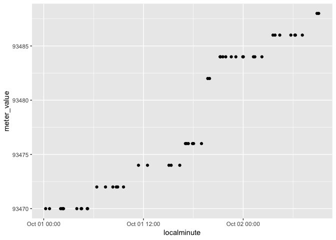
For the Markdown table/pipe-delimited version, you can use lubridate::ymd_hm (there are no seconds), which is equivalent to lubridate::parse_date_time with "Ymd HM" for the orders parameter. No time zones are supplied with this data, so this may be off from the real-world data:

library(tidyverse)

PlotD <- structure(list(localminute = c("1/10/2015 0:14", "1/10/2015 0:42", "1/10/2015 2:02", "1/10/2015 2:12", "1/10/2015 2:20", "1/10/2015 2:23", "1/10/2015 3:59", "1/10/2015 4:30", "1/10/2015 4:34", "1/10/2015 5:14", "1/10/2015 5:17", "1/10/2015 6:23", "1/10/2015 7:26", "1/10/2015 8:19", "1/10/2015 8:44", "1/10/2015 8:54", "1/10/2015 9:36", "1/10/2015 11:24", "1/10/2015 12:29", "1/10/2015 15:04", "1/10/2015 15:20", "1/10/2015 16:22", "1/10/2015 17:03", "1/10/2015 17:11", "1/10/2015 17:24", "1/10/2015 17:54", "1/10/2015 18:02", "1/10/2015 18:59", "1/10/2015 19:44", "1/10/2015 19:57", "1/10/2015 21:13", "1/10/2015 21:16", "1/10/2015 21:33", "1/10/2015 21:54", "1/10/2015 22:34", "1/10/2015 23:07", "1/10/2015 23:57", "2/10/2015 0:01", "2/10/2015 1:14", "2/10/2015 1:24", "2/10/2015 2:15", "2/10/2015 3:35", "2/10/2015 3:50", "2/10/2015 4:24", "2/10/2015 5:44", "2/10/2015 6:13", "2/10/2015 6:17", "2/10/2015 7:07", "2/10/2015 8:53", "2/10/2015 9:05"), 
                        dataid = c(35L, 35L, 35L, 35L, 35L, 35L, 35L, 35L, 35L, 35L, 35L, 35L, 35L, 35L, 35L, 35L, 35L, 35L, 35L, 35L, 35L, 35L, 35L, 35L, 35L, 35L, 35L, 35L, 35L, 35L, 35L, 35L, 35L, 35L, 35L, 35L, 35L, 35L, 35L, 35L, 35L, 35L, 35L, 35L, 35L, 35L, 35L, 35L, 35L, 35L), 
                        meter_value = c(93470L, 93470L, 93470L, 93470L, 93470L, 93470L, 93470L, 93470L, 93470L, 93470L, 93470L, 93472L, 93472L, 93472L, 93472L, 93472L, 93472L, 93474L, 93474L, 93474L, 93474L, 93474L, 93476L, 93476L, 93476L, 93476L, 93476L, 93476L, 93482L, 93482L, 93484L, 93484L, 93484L, 93484L, 93484L, 93484L, 93484L, 93484L, 93484L, 93484L, 93484L, 93486L, 93486L, 93486L, 93486L, 93486L, 93486L, 93486L, 93488L, 93488L)), 
                   class = "data.frame", row.names = c(NA, -50L))

PlotD %>% 
    mutate(localminute = lubridate::dmy_hm(localminute)) %>% 
    ggplot(aes(x = localminute, y = meter_value)) + 
    geom_point()
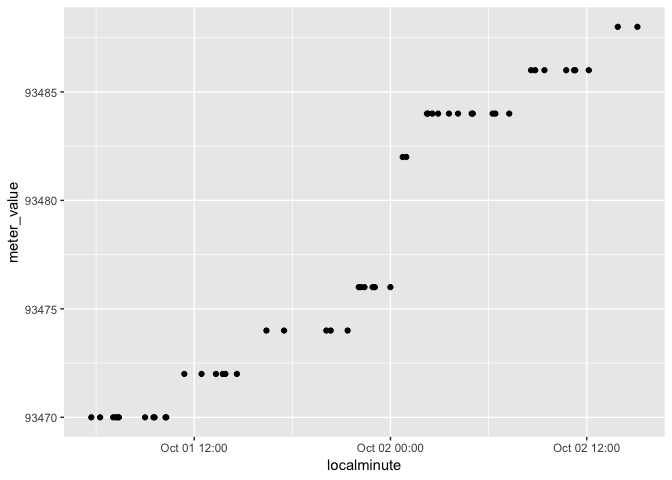
For the CSV formatted one, you need to use decimal seconds and a timezone offset, which lubridate's shortcut parsers can't do, but its full-bore parse_date_time can:

library(tidyverse)

PlotD <- structure(list(localminute = c("2015-10-01 00:14:44.119722-06", "2015-10-01 00:42:34-05", "2015-10-01 02:02:37-05", "2015-10-01 02:12:38-05", "2015-10-01 02:20:36-05", "2015-10-01 02:23:39-05", "2015-10-01 03:59:41-05", "2015-10-01 04:30:40-05", "2015-10-01 04:34:37-05", "2015-10-01 05:14:35-05", "2015-10-01 05:17:32-05", "2015-10-01 06:23:36.547408-05", "2015-10-01 07:26:51-05", "2015-10-01 08:19:40-05", "2015-10-01 08:44:40-05", "2015-10-01 08:54:30-05", "2015-10-01 09:36:34-05", "2015-10-01 11:24:52-05", "2015-10-01 12:29:40-05", "2015-10-01 15:04:40-05", "2015-10-01 15:20:41-05", "2015-10-01 16:22:43-05", "2015-10-01 17:03:44-05", "2015-10-01 17:11:38-05", "2015-10-01 17:24:32-05", "2015-10-01 17:54:31-05", "2015-10-01 18:02:35-05", "2015-10-01 18:59:38-05", "2015-10-01 19:44:49-05", "2015-10-01 19:57:48-05", "2015-10-01 21:13:46-05", "2015-10-01 21:16:44-05", "2015-10-01 21:33:31-05", "2015-10-01 21:54:36-05", "2015-10-01 22:34:32-05", "2015-10-01 23:07:40-05", "2015-10-01 23:57:49-05", "2015-10-02 00:01:51-05", "2015-10-02 01:14:44-05", "2015-10-02 01:24:44-05", "2015-10-02 02:15:34-05", "2015-10-02 03:35:41-05", "2015-10-02 03:50:46-05", "2015-10-02 04:24:51-05", "2015-10-02 05:44:41-05", "2015-10-02 06:13:39-05", "2015-10-02 06:17:37-05", "2015-10-02 07:07:29-05", "2015-10-02 08:53:46-05", "2015-10-02 09:05:45.520209-06"), 
                        dataid = c(35L, 35L, 35L, 35L, 35L, 35L, 35L, 35L, 35L, 35L, 35L, 35L, 35L, 35L, 35L, 35L, 35L, 35L, 35L, 35L, 35L, 35L, 35L, 35L, 35L, 35L, 35L, 35L, 35L, 35L, 35L, 35L, 35L, 35L, 35L, 35L, 35L, 35L, 35L, 35L, 35L, 35L, 35L, 35L, 35L, 35L, 35L, 35L, 35L, 35L), 
                        meter_value = c(93470L, 93470L, 93470L, 93470L, 93470L, 93470L, 93470L, 93470L, 93470L, 93470L, 93470L, 93472L, 93472L, 93472L, 93472L, 93472L, 93472L, 93474L, 93474L, 93474L, 93474L, 93474L, 93476L, 93476L, 93476L, 93476L, 93476L, 93476L, 93482L, 93482L, 93484L, 93484L, 93484L, 93484L, 93484L, 93484L, 93484L, 93484L, 93484L, 93484L, 93484L, 93486L, 93486L, 93486L, 93486L, 93486L, 93486L, 93486L, 93488L, 93488L)), 
                   class = "data.frame", row.names = c(NA, -50L))

PlotD %>% 
    mutate(localminute = lubridate::parse_date_time(localminute, 'Ymd HMS!z!')) %>% 
    ggplot(aes(x = localminute, y = meter_value)) + 
    geom_point()
For documentation, start with ?strptime. That function doesn't get used much anymore (it returns POSIXlt class, which [deliberately] doesn't play nice in tibbles), but it is where base R's date-time parsing token system (used in as.POSIXct and as.Date, as well) is documented. Next read ?lubridate::parse_date_time, which shows that lubridate is a riff on the basic strptime format that in some contexts does not require the % and delimiter characters to be supplied. It also includes some other special tokens, including the %S! and %z! used above.

1 Like

Hi May,
I hope we can help. @prosoitos gave a good summary of what we've figured out so far. It would be helpful if we could learn more about the data source to confirm that those guesses about interpreting the data are correct.

From this warning message

Warning message:
All formats failed to parse. No formats found.

we can see that your localminute variable is not getting interpreted correctly by lubridate for ANY rows. We need to fix that first before the rest can work. I suspect the issue is that it doesn't know what to do with the "-05" and "-06" that appear at the end of the localminute variable. I think @jcblum is probably right about those being time zone offsets, so you should confirm that in order to have confidence in what you find. For the moment, let's assume that's right and see what happens...

Below I load the data into a dataframe (using your Apr 15 email plus datapasta). Then I check how long each localminute entry is, so that I can split out the last two characters from the rest. There are slicker ways to do this using "regex", but hopefully this makes the process legible. Once I've split localminute into two pieces, I use the first piece to give lubridate a clean time in "year month day hour minute second" order, and then I add what I assume is offset hours to that.

End result seems plausible, but that might be a coincidence...

data_20180415 <- data.frame(
   localminute = c("2015-10-01 00:14:44.119722-06", "2015-10-01 00:42:34-05",
                   "2015-10-01 02:02:37-05", "2015-10-01 02:12:38-05",
                   "2015-10-01 02:20:36-05", "2015-10-01 02:23:39-05",
                   "2015-10-01 03:59:41-05", "2015-10-01 04:30:40-05", "2015-10-01 04:34:37-05",
                   "2015-10-01 05:14:35-05", "2015-10-01 05:17:32-05",
                   "2015-10-01 06:23:36.547408-05", "2015-10-01 07:26:51-05",
                   "2015-10-01 08:19:40-05", "2015-10-01 08:44:40-05", "2015-10-01 08:54:30-05",
                   "2015-10-01 09:36:34-05", "2015-10-01 11:24:52-05",
                   "2015-10-01 12:29:40-05", "2015-10-01 15:04:40-05",
                   "2015-10-01 15:20:41-05", "2015-10-01 16:22:43-05", "2015-10-01 17:03:44-05",
                   "2015-10-01 17:11:38-05", "2015-10-01 17:24:32-05",
                   "2015-10-01 17:54:31-05", "2015-10-01 18:02:35-05",
                   "2015-10-01 18:59:38-05", "2015-10-01 19:44:49-05", "2015-10-01 19:57:48-05",
                   "2015-10-01 21:13:46-05", "2015-10-01 21:16:44-05",
                   "2015-10-01 21:33:31-05", "2015-10-01 21:54:36-05", "2015-10-01 22:34:32-05",
                   "2015-10-01 23:07:40-05", "2015-10-01 23:57:49-05",
                   "2015-10-02 00:01:51-05", "2015-10-02 01:14:44-05",
                   "2015-10-02 01:24:44-05", "2015-10-02 02:15:34-05", "2015-10-02 03:35:41-05",
                   "2015-10-02 03:50:46-05", "2015-10-02 04:24:51-05",
                   "2015-10-02 05:44:41-05", "2015-10-02 06:13:39-05", "2015-10-02 06:17:37-05",
                   "2015-10-02 07:07:29-05", "2015-10-02 08:53:46-05",
                   "2015-10-02 09:05:45.520209-06"),
        dataid = c(35L, 35L, 35L, 35L, 35L, 35L, 35L, 35L, 35L, 35L, 35L, 35L,
                   35L, 35L, 35L, 35L, 35L, 35L, 35L, 35L, 35L, 35L, 35L, 35L,
                   35L, 35L, 35L, 35L, 35L, 35L, 35L, 35L, 35L, 35L, 35L, 35L,
                   35L, 35L, 35L, 35L, 35L, 35L, 35L, 35L, 35L, 35L, 35L, 35L, 35L,
                   35L),
   meter_value = c(93470L, 93470L, 93470L, 93470L, 93470L, 93470L, 93470L,
                   93470L, 93470L, 93470L, 93470L, 93472L, 93472L, 93472L,
                   93472L, 93472L, 93472L, 93474L, 93474L, 93474L, 93474L, 93474L,
                   93476L, 93476L, 93476L, 93476L, 93476L, 93476L, 93482L, 93482L,
                   93484L, 93484L, 93484L, 93484L, 93484L, 93484L, 93484L,
                   93484L, 93484L, 93484L, 93484L, 93486L, 93486L, 93486L, 93486L,
                   93486L, 93486L, 93486L, 93488L, 93488L)
)


data_20180415_split <-
  data_20180415 %>%
  mutate(lm_length = nchar(localminute %>% as.character()),
         lm_base   = localminute %>% substr(0, lm_length-3),
         lm_offset = localminute %>% substr(lm_length-1, lm_length) %>% as.integer) %>%
  mutate(lm_norm   = lubridate::ymd_hms(lm_base) + lubridate::dhours(lm_offset))


ggplot(data_20180415_split, 
       aes(x = lm_norm, y = meter_value)) + 
  geom_point() + ggtitle("meter value for dataID=35") + 
  theme(axis.text.x = element_text(angle = 90, hjust = 1))

Hi Alistaire,

Thanks for your reply. I tried with your suggested code, i can get same output as yours. If you dont mind, could you explain me the meaning of this code below

PlotD <- structure(list(localminute = c("2015-10-01 00:14:44.119722-06", "2015-10-01 00:42:34-05", "2015-10-01 02:02:37-05", "2015-10-01 02:12:38-05", "2015-10-01 02:20:36-05", "2015-10-01 02:23:39-05", "2015-10-01 03:59:41-05", "2015-10-01 04:30:40-05", "2015-10-01 04:34:37-05", "2015-10-01 05:14:35-05", "2015-10-01 05:17:32-05", "2015-10-01 06:23:36.547408-05", "2015-10-01 07:26:51-05", "2015-10-01 08:19:40-05", "2015-10-01 08:44:40-05", "2015-10-01 08:54:30-05", "2015-10-01 09:36:34-05", "2015-10-01 11:24:52-05", "2015-10-01 12:29:40-05", "2015-10-01 15:04:40-05", "2015-10-01 15:20:41-05", "2015-10-01 16:22:43-05", "2015-10-01 17:03:44-05", "2015-10-01 17:11:38-05", "2015-10-01 17:24:32-05", "2015-10-01 17:54:31-05", "2015-10-01 18:02:35-05", "2015-10-01 18:59:38-05", "2015-10-01 19:44:49-05", "2015-10-01 19:57:48-05", "2015-10-01 21:13:46-05", "2015-10-01 21:16:44-05", "2015-10-01 21:33:31-05", "2015-10-01 21:54:36-05", "2015-10-01 22:34:32-05", "2015-10-01 23:07:40-05", "2015-10-01 23:57:49-05", "2015-10-02 00:01:51-05", "2015-10-02 01:14:44-05", "2015-10-02 01:24:44-05", "2015-10-02 02:15:34-05", "2015-10-02 03:35:41-05", "2015-10-02 03:50:46-05", "2015-10-02 04:24:51-05", "2015-10-02 05:44:41-05", "2015-10-02 06:13:39-05", "2015-10-02 06:17:37-05", "2015-10-02 07:07:29-05", "2015-10-02 08:53:46-05", "2015-10-02 09:05:45.520209-06"),
dataid = c(35L, 35L, 35L, 35L, 35L, 35L, 35L, 35L, 35L, 35L, 35L, 35L, 35L, 35L, 35L, 35L, 35L, 35L, 35L, 35L, 35L, 35L, 35L, 35L, 35L, 35L, 35L, 35L, 35L, 35L, 35L, 35L, 35L, 35L, 35L, 35L, 35L, 35L, 35L, 35L, 35L, 35L, 35L, 35L, 35L, 35L, 35L, 35L, 35L, 35L),
meter_value = c(93470L, 93470L, 93470L, 93470L, 93470L, 93470L, 93470L, 93470L, 93470L, 93470L, 93470L, 93472L, 93472L, 93472L, 93472L, 93472L, 93472L, 93474L, 93474L, 93474L, 93474L, 93474L, 93476L, 93476L, 93476L, 93476L, 93476L, 93476L, 93482L, 93482L, 93484L, 93484L, 93484L, 93484L, 93484L, 93484L, 93484L, 93484L, 93484L, 93484L, 93484L, 93486L, 93486L, 93486L, 93486L, 93486L, 93486L, 93486L, 93488L, 93488L)),
class = "data.frame", row.names = c(NA, -50L))

Please correct me, if I am wrong.
You used "structure and list" for arranging local minute data into this format "Ymd Hms" ?

Your suggested code display all the 50 data of local minute. But, what if there are 1000 or more local minute data? I feel that the code will be very messy, if all the large local minute data display.

Why dataid and meter_value is assigned to "c" function and why you put "L" for all dataID and meter_value?

What command should I for those large data which needs to read from csv file and straight away plot in R?

class= "data.frame" #what I know what this stands for?
row.names =c (NA, -50L) # what is the meaning of this?

Sorry, that's the result of calling dput on the data frame, which returns code that generates the data in exactly the same format on any computer. You won't need to run that on your actual data, where you'll can use the appropriate read* function.

Hi Jcblum,

Sorry for late reply. My supervisor gave me the csv file, to analyze the data.

We are not concerned about the extra precision on the seconds and time zone offsets, that is why, I would like to remove "-nn" values, when I plot.

I tried "str(PlotD)" and output as below:

> PlotD <- read.csv("test_R.csv") #data in test_R.csv remain the same as I stated the data in comment no10.

> str(PlotD)
'data.frame':	50 obs. of  3 variables:
 $ localminute: Factor w/ 50 levels "2015-10-01 00:14:44.119722-06",..: 1 2 3 4 5 6 7 8 9 10 ...
 $ dataid     : int  35 35 35 35 35 35 35 35 35 35 ...
 $ meter_value: int  93470 93470 93470 93470 93470 93470 93470 93470 93470 93470 ...

However, my actual csv file that I m going to analyze, the str output as below

>  FYP <- read.csv("dataport_oct2015-mar2016_org.csv")
> str(FYP)
'data.frame':	1584823 obs. of  3 variables:
 $ localminute: Factor w/ 1544152 levels "2015-10-01 00:00:10-05",..: 1 2 3 4 4 5 6 7 8 9 ...
 $ dataid     : int  739 8890 6910 3635 1507 5810 484 6910 6910 5810 ...
 $ meter_value: int  88858 197164 179118 151318 390354 97506 99298 179118 179118 97506 ...

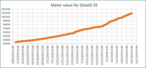
I am concerned that, we could not see the X-axis, if I plot all data (1,584,823 data). How should I plot all data, by scaling X-axis (24 hour gap), as the image below, that I plotted in excel
image