How to make a longer and clearer legend scale bar

[Ellenz]

The original post is here: How to enlarge the size of each sub-panel with common scale bar - #22 by andresrcs

I use the optional code below to display the continuous variable. How to increase the length of the scale bar and to display more colors? For example, if my P(mm) spans a large range, how to display the data? Right now, my scale bar has a small range. Thanks for your help.

scale_fill_distiller('P (mm)',palette='Spectral') +
scale_color_gradientn(name='P (mm)',colours = rainbow(7))+

[Ellenz]

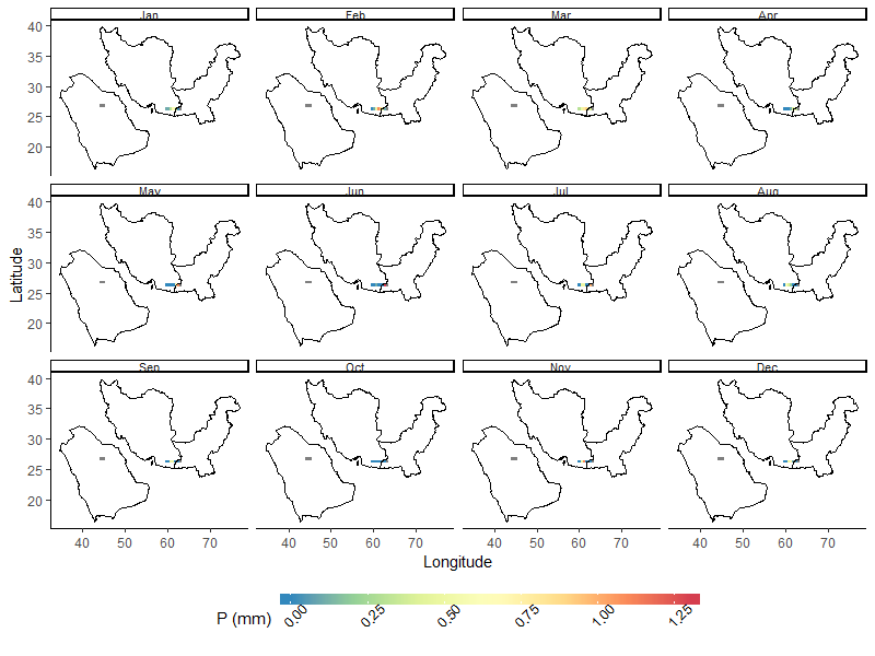
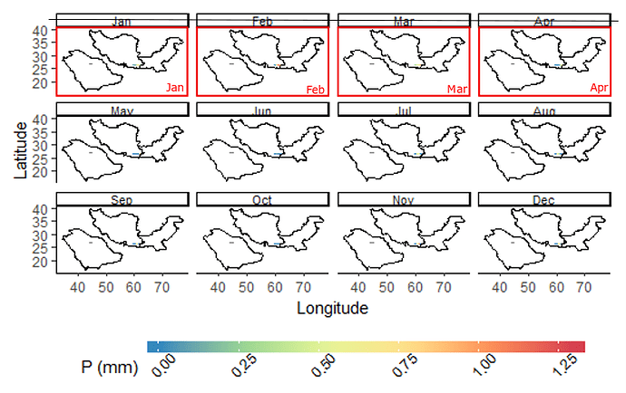
Besides (1) increasing the colors of the legend bar, or making the colors in the figure more distinct, I have another question about how to change the shape of the color bar.

I would like to make the legend bar longer and narrower, so that there will be more colors to show. I use the code and the source below, but could not make it to work in my case. Thanks.
source: Continuous colour bar guide — guide_colourbar • ggplot2

guides(fill = guide_colourbar(barwidth = 0.5, barheight = 10))

And (2) how to display months as "Jan, Feb, Mar, Apr, ..." rather than "1, 2, 3, 4, ..."? (3) How to add all four frames for each monthly sub-panel? This means that I want to have the left, bottom, and right frames, rather than leaving them out. The datasets and code are below:

df1 = data.frame( lon= c(59.75, 60.25, 60.75, 61.25, 61.75, 62.25 ,62.75, 63.25, 44.25, 44.75, 45.25),
lat = c(26.25, 26.25, 26.25, 26.25, 26.25, 26.25, 26.25, 26.25, 26.75, 26.75, 26.75),
P = c(0.1, 0.1, 0.3, 0.7, 0.6, 0.4, 0.02, NA, NA, NA, NA) )

df2 = data.frame( lon= c(59.75, 60.25, 60.75, 61.25, 61.75, 62.25 ,62.75, 63.25, 44.25, 44.75, 45.25),
lat = c(26.25, 26.25, 26.25, 26.25, 26.25, 26.25, 26.25, 26.25, 26.75, 26.75, 26.75),
P= c(0, 0.1, 0.5, 1.1, 0.9, 0.5, 0.1, NA, NA, NA, NA) )

df3= data.frame( lon= c(59.75, 60.25, 60.75, 61.25, 61.75, 62.25 ,62.75, 63.25, 44.25, 44.75, 45.25),
lat = c(26.25, 26.25, 26.25, 26.25, 26.25, 26.25, 26.25, 26.25, 26.75, 26.75, 26.75),
P= c(0.3, 0.3, 0.5, 0.8, 0.9, 0.6, 0.4, NA, NA, NA, NA))

df4= data.frame( lon =c(59.75, 60.25, 60.75, 61.25, 61.75, 62.25 ,62.75, 63.25, 44.25, 44.75, 45.25),
lat= c(26.25, 26.25, 26.25, 26.25, 26.25, 26.25, 26.25, 26.25, 26.75, 26.75, 26.75),
P= c(0, 0, 0, 0.1, 0.4, 0.6, 0.3, NA, NA, NA, NA))

df5= data.frame( lon =c(59.75, 60.25, 60.75, 61.25, 61.75, 62.25 ,62.75, 63.25, 44.25, 44.75, 45.25),
lat= c(26.25, 26.25, 26.25, 26.25, 26.25, 26.25, 26.25, 26.25, 26.75, 26.75, 26.75),
P= c(0, 0, 0, 0, 0, 0.7, 1.1, NA, NA, NA, NA))

df6 = data.frame( lon =c(59.75, 60.25, 60.75, 61.25, 61.75, 62.25 ,62.75, 63.25, 44.25, 44.75, 45.25),
lat= c(26.25, 26.25, 26.25, 26.25, 26.25, 26.25, 26.25, 26.25, 26.75, 26.75, 26.75),
P= c(0, 0, 0.1, 0, 0, 0, 1.3, NA, NA, NA, NA))

df7= data.frame( lon =c(59.75, 60.25, 60.75, 61.25, 61.75, 62.25 ,62.75, 63.25, 44.25, 44.75, 45.25),
lat= c(26.25, 26.25, 26.25, 26.25, 26.25, 26.25, 26.25, 26.25, 26.75, 26.75, 26.75),
P= c(0, 0, 0.5, 0.5, 0, 0, 1, NA, NA, NA, NA))

df8 = data.frame( lon =c(59.75, 60.25, 60.75, 61.25, 61.75, 62.25 ,62.75, 63.25, 44.25, 44.75, 45.25),
lat= c(26.25, 26.25, 26.25, 26.25, 26.25, 26.25, 26.25, 26.25, 26.75, 26.75, 26.75),
P= c(0, 0.6, 0.4, 0.2, 0, 0, 0, NA, NA, NA, NA))

df9= data.frame( lon =c(59.75, 60.25, 60.75, 61.25, 61.75, 62.25 ,62.75, 63.25, 44.25, 44.75, 45.25),
lat= c(26.25, 26.25, 26.25, 26.25, 26.25, 26.25, 26.25, 26.25, 26.75, 26.75, 26.75),
P= c(0, 0, 0.5, 0.5, 0, 0, 0, NA, NA, NA, NA))

df10 = data.frame( lon =c(59.75, 60.25, 60.75, 61.25, 61.75, 62.25 ,62.75, 63.25, 44.25, 44.75, 45.25),
lat= c(26.25, 26.25, 26.25, 26.25, 26.25, 26.25, 26.25, 26.25, 26.75, 26.75, 26.75),
P= c(0, 0, 0, 0, 0, 0, 0, NA, NA, NA, NA))

df11 = data.frame( lon =c(59.75, 60.25, 60.75, 61.25, 61.75, 62.25 ,62.75, 63.25, 44.25, 44.75, 45.25),
lat= c(26.25, 26.25, 26.25, 26.25, 26.25, 26.25, 26.25, 26.25, 26.75, 26.75, 26.75),
P= c(0, 0, 0.5, 1.1, 0, 0, 0, NA, NA, NA, NA))

df12= data.frame( lon =c(59.75, 60.25, 60.75, 61.25, 61.75, 62.25 ,62.75, 63.25, 44.25, 44.75, 45.25),
lat= c(26.25, 26.25, 26.25, 26.25, 26.25, 26.25, 26.25, 26.25, 26.75, 26.75, 26.75),
P= c(0, 0, 0.5, 0.7, 0.1, 0.1, 0, NA, NA, NA, NA))
library(tidyverse)

bind_rows(df1,df2,df3,df4,df5,df6,df7,df8,df9,df10,df11,df12,.id = "Month") %>%
mutate(Month = as.numeric(Month)) %>% # Convert the categorical variable to numeric
ggplot(aes(lon, lat, fill = P)) +
geom_tile() +
theme_classic() +
scale_fill_distiller('P (mm)',palette='Spectral') +
borders('world', xlim=range(df1$lon), ylim=range(df1$lat), colour='black') +
#coord_quickmap(xlim=range(df1$lon), ylim=range(df1$lat)) + # The proportions of the facets are afected by this limits
facet_wrap(vars(Month)) + xlab('Longitude') + ylab('Latitude') +
theme(legend.position = "bottom",
legend.text = element_text(angle = 45),
strip.text.x = element_text(size = 8, margin = margin(0, 0, 0, 0, "cm")))

Sorry, I tried to use reprex but got the error below:

reprex()
Rendering reprex...
Error in curl::curl_fetch_memory(url, handle = handle) :
Timeout was reached: Connection timed out after 10000 milliseconds

[Ellenz]

Could someone help me with this? I really appreciate it. I understand that it maybe because I did not use reprex to post it, but there was the error message also. Thanks again for your help.

[pafmax]

Hi, This should help with question 1 and 3, don't understand what you're after on 3, though:

data <- bind_rows(df1, df2, df3,  df4, df5, df6, df7, df8, df9, df10, df11, df12, .id = "Month") %>%
    mutate(Month = lubridate::month(as.numeric(Month), label = TRUE)) 

ggplot(data, aes(lon, lat, fill = P)) +
    geom_tile() +
    theme_classic() +
    scale_fill_distiller('P (mm)', palette = 'Spectral') +
    borders(
        'world',
        xlim = range(df1$lon),
        ylim = range(df1$lat),
        colour = 'black'
    ) +
    facet_wrap(. ~ Month) +
    xlab('Longitude') +
    ylab('Latitude') +
    theme(
        legend.position = "bottom",
        legend.text = element_text(angle = 45),
        strip.text.x = element_text(size = 8, margin = margin(0, 0, 0, 0, "cm"))
    ) +
    guides(fill = guide_colorbar(barwidth = 20, barheight = 0.5))

This is what I get:

Cheers

[Ellenz]

Thanks for your help. For the other question, I meant that how to have the rectangular borders as the red borders in the attached figure? I manually added them, but thought there may be a way in the code. Using the original code, the borders are missing.

Also, the boxes with "Jan, Feb, Mar, ..." take too much space, so is there a way to remove these boxes, but denote "Jan, Feb, Mar, ..." in the blank spots around the main figure? Like in the attached figure. Thanks.