How to deal with weighted survey data?

I am trying to analyze nationally representative data from the World Bank's Living Standard Measurement Survey. It has a weight variable that has to be applied to make the data nationally representative. I applied the weight to descriptive statistics and was able to replicate the approximate results they reported. However, I'm very confused and don't know how to handle these weights within different package models. I applied these weights to the data using the Survey package, but only a limited number of packages support svydesign object from Survey package.

I have read this:

When I used the uncount function, the data ended with more than 1 million cases, which is heavy to analyze.

Also tried to apply weights to each variable prior to modelling (panel) but was confused about how to apply them to categorical variables.

How can I use these weights?

Hi, welcome!

We don't really have enough info to help you out. Could you ask this with a minimal REPRoducible EXample (reprex)? A reprex makes it much easier for others to understand your issue and figure out how to help.

If you've never heard of a reprex before, you might want to start by reading this FAQ:

Thank you @nirgrahamuk .
Here is the problem that I'm facing: I want to apply the weight (pw variable) globally. For example, here I want to construct a summary table using gtsummary. I'm able to do what I wanted when I use the uncount function from the package from the tidyverse family. Is there any better alternative to doing this? Since the real data has more than 100 million observations when uncounted, it is impossible to use that technique.

# Example data;
df <- data.frame(id = c(1, 2, 3, 1, 2, 3, 1, 2, 3),
           pw = c(207, 188,41,32,137,86,170,213,135),
           sex = as.factor(c("Male","Female","Female","Male","Male",
                             "Female","Female","Male","Male")),
           location = as.factor(c("Rural","Rural","Urban","Urban","Urban",
                             "Urban","Rural","Urban","Urban")),
           age = c(39, 34, 44, 37, 53, 61, 57, 46, 54),
           bmi = c(21, 18, 20, 17, 22, 24, 25, 19, 26))

library(tidyverse)      # For data manipulation
library(gtsummary)      # To make summary table
                        # You need it only if you run the #'ed codes

# The table that I want to weight with pw variable
# Below the code

# df %>% select(!c(pw, id)) %>% 
        # tbl_summary(by = sex, percent = "row", 
                    # statistic = list(all_continuous() ~ "{mean} ({sd})",
                                    # all_categorical() ~ "({p}%)"),
                   # type = c(age, bmi) ~ "continuous")

f.data <- df %>% filter(sex == "Female")# To show what I want to get
mean(f.data$age)                        # Which is being shown in the table
#> [1] 49
weighted.mean(f.data$age, f.data$pw)    # The mean that I want in table
#> [1] 47.69485

# How can apply the weight globally without using uncount function?
# This is the final result I want without uncount since the real data
# has more than 300 million observation when uncounted

# df %>% uncount(pw) %>% select(!id) %>% 
        # tbl_summary(by = sex, percent = "row", 
                    # statistic = list(all_continuous() ~ "{mean} ({sd})",
                                    # all_categorical() ~ "({p}%)"),
                    # type = c(age, bmi) ~ "continuous")

Created on 2023-04-20 with reprex v2.0.2

The example codes for the table that I want to construct were preceded by # so you can remove them and run.

Any help is much appreciated!

Great reprex.

Here's a solution that exploits the structure returned by tbl_summary to locate where the mean needs changing to weighted.mean and it doesn't involve tidyr::uncount() at all.

library(gtsummary)
#> #BlackLivesMatter

# pattern to detect part of a string before a space or (

pat <- "^.* "

# obtain pw weighted mean age for a sex

get_wm <- function(x) {round(weighted.mean(d[which(d$sex == x),5],
                                           d[which(d$sex == x),2]),0)
}

d <- data.frame(id = c(1, 2, 3, 1, 2, 3, 1, 2, 3),
                 pw = c(207, 188,41,32,137,86,170,213,135),
                 sex = as.factor(c("Male","Female","Female","Male","Male",
                                   "Female","Female","Male","Male")),
                 location = as.factor(c("Rural","Rural","Urban","Urban","Urban",
                                        "Urban","Rural","Urban","Urban")),
                 age = c(39, 34, 44, 37, 53, 61, 57, 46, 54),
                 bmi = c(21, 18, 20, 17, 22, 24, 25, 19, 26))

# prepare table with unweighted mean age

o <- d[,-c(1,2)] |> 
  tbl_summary(by = sex, percent = "row",
              statistic = list(all_continuous() ~ "{mean} ({sd})",
                               all_categorical() ~ "({p}%)"),
              type = c(age, bmi) ~ "continuous")


# inspect
# enter this to see where the target object was found
# str(o) 

# substitute weighted mean ages in summary table

o$table_body$stat_1[4] <- sub(pat,paste(get_wm("Female"),""),o$table_body$stat_1[4])
o$table_body$stat_2[4] <- sub(pat,paste(get_wm("Male"),""),o$table_body$stat_2[4])

Created on 2023-04-22 with reprex v2.0.2

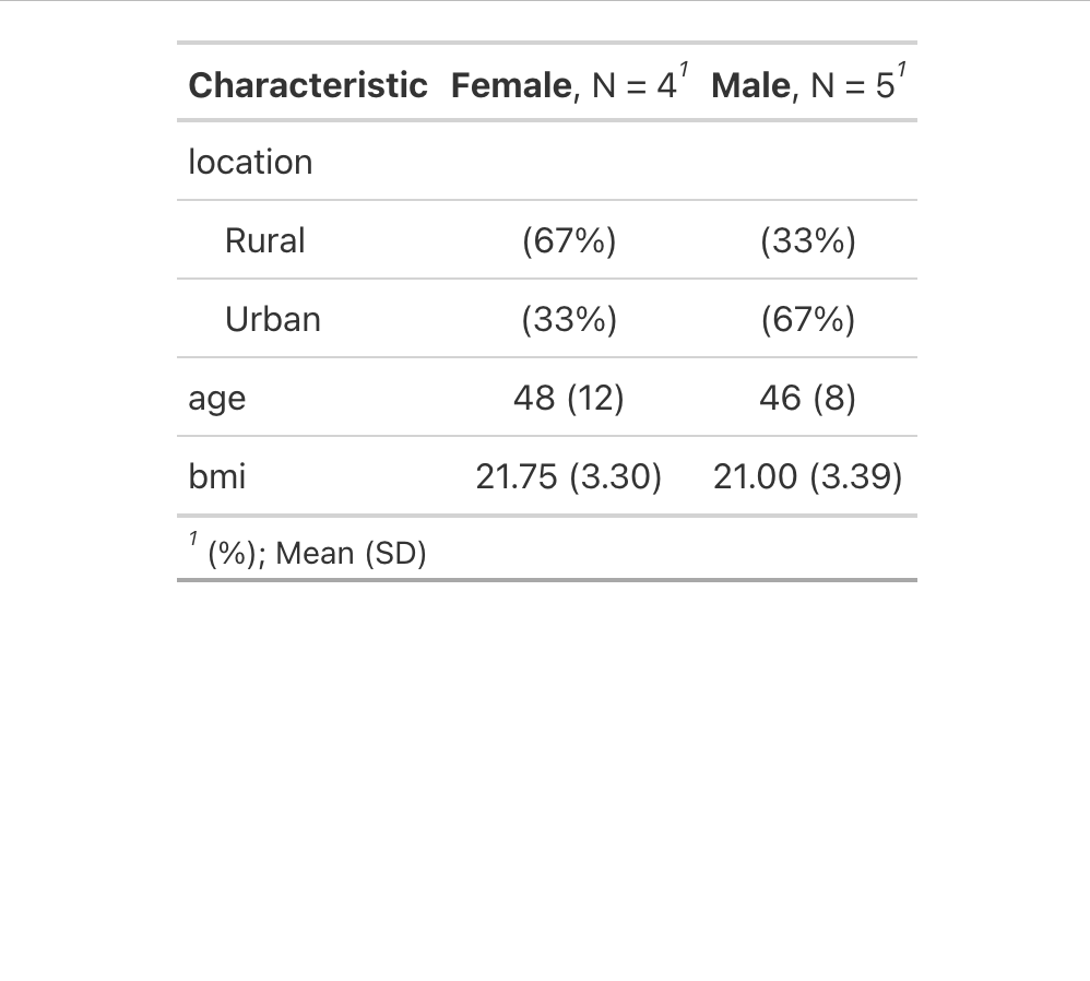
gtsummary produces html markup that doesn't display well here, so here is the before
table as an image

with a mean of 49, and here is the after table with a mean of 48 as an image

Rationale: school algebra—f(x)=y where

x is the object at hand, in this case the data frame d.
y is the desired object, a tbl_summary nested lists with a print method to format as the presentation table created with the first tbl_summary() call *with the exception that the age row display the return value of weighted.mean() rather than mean().
f is the chain of functions (composite function) to transform x into y.

Most of the work is already done by the first tbl_summary() call. Then, using str(o) (o is for object, as d is for data frame) we find

 str(o)
# List of 8
#  $table_body   : tibble [5 Ă— 7] (S3: tbl_df/tbl/data.frame)
# {snip}

o is a named list and its first element, named table_body is a tibble and we can extract that by name o$table_body. Scrolling down we come to what we are looking for in terms of where the values are to be changed.

  ..$ stat_1   : chr [1:5] NA "(67%)" "(33%)" "49 (12)" ...
  ..$ stat_2   : chr [1:5] NA "(33%)" "(67%)" "46 (8)" ...

which we can refer to as o$table_body$stat_1 and ...stat_2.

Let's examine the first

o$table_body$stat_1
# [1] NA             "(67%)"        "(33%)"       
# [4] "49 (12)"      "21.75 (3.30)"

It's a five element character vector, and the fourth element, which contains the mean value to be changed is element 4, which is the character string "49 (12)" All that needs to be changed is the value before the space. (If sd is to be similarly adjusted, both would need be.)

Within that string are the characters 49 separated by a space character from the following characters enclosed in (). The first can be identified by the pat regular expression—zero or more characters at the beginning followed by a space. Having drilled down to the mean value to be replace, there remains only the replacement.

get_wm does the weighted.mean() calculation for the entire data frame by Sex without the trouble of uncount(), and that is used as the replacement in sub(). The final fussiness of paste() is just to restore the space.

1 Like

Thank you so much, @technocrat, for your clear and to-the-point explanation.

Yeah, this is what I was looking for!

1 Like

This topic was automatically closed 7 days after the last reply. New replies are no longer allowed.

If you have a query related to it or one of the replies, start a new topic and refer back with a link.