Graph Annotator
Authors: Matthew Montero
Abstract: To bridge the gap between programmers and non-programmers, this self-service shiny application provides the target user, the non-programmer, the ability to upload graphs created by the R package ggplot2 and interactively annotate with text and geometrics.
At any point, the user can download the annotated graph, in a selected format, and/or the reproduceable R code which may be handed back to the programmer to integrate.
Full Description:
Background
Like other industries, in pharmaceuticals, teams are made up of a mixture of skills sets all having a common goal --- creating reproducible and high-quality content.
While creating requirements to develop content has its advantages, the ad-hoc nature of annotations creates a bottleneck in some workflows. While still in its infancy, this application is an attempt to reduce this bottleneck.
The core of the shiny application is based on the mathematical concept functional decomposition, which refers broadly to the process of resolving a functional relationship into its constituent parts in such a way that the original function can be reconstructed from those parts. In other words, recursively breaking down a function call to its’ parts.
For example, the function call sum(x = 1, y = 2) can be broken down to its function = "sum" and arguments x = 1, and y = 2.
Let’s represent the functional decomposition of this function call using a list:
list(.fn = 'sum',
     x= 1,
     y= 2)
In a similar matter, this concept can be applied to function calls within functions such as sum(x = prod(2,3), y = 2).
The functional decomposition object is static, which is used to create both the graph, by composing the function into a call and evaluating it, and R code, saving the un-evaluated call. Note, the latter is simply a byproduct of the process rather than the focus.
While not covered in this application, the object representing the decomposed function has many more uses by first converting it into a JSON file. The simple conversation now opens the door to API requests, URL queries, and many others.
Getting Started
The application is split into three steps: 1 Upload Graph, 2 Visualize, and 3 Publish.
In the first step, Upload Graph, you can choose from the demo examples taken from the ggplot2 references or upload your own .Rds file:
library(ggplot2)
gg <- ggplot(mtcars, aes(x = wt, y = mpg)) + geom_point()
saveRDS(gg, file = 'ex.Rds')
Note, only native ggplot2 functionality is currently supported.
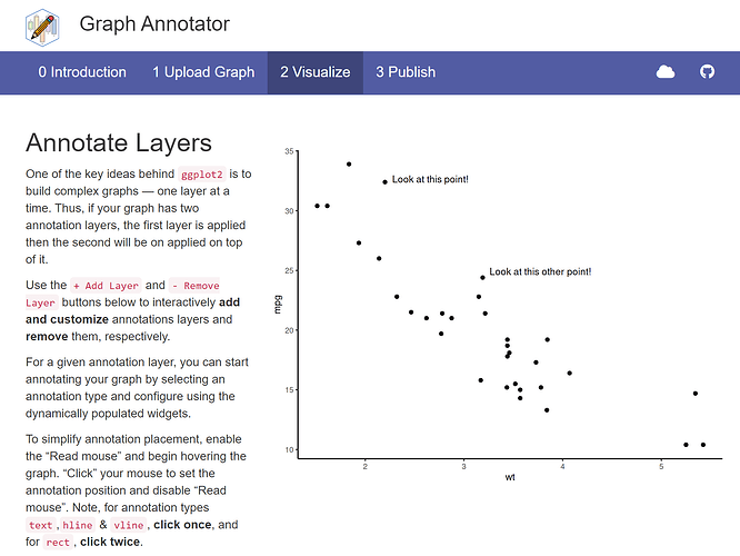
In the second step, Visualize, you can start annotating your graph by selecting an annotation type. Based on the select type, configure your annotation using the populated widgets. To simplify annotation placement, enable the “Read mouse” and begin hovering the graph. “Click” once you have moved your annotation to the desired location.
Finally, in the third step, Publish, you can save your graph to an image file and/or save the reproducible R code.
Keywords: ggplot2, visualization, annotation
Shiny app: https://matthew-montero.shinyapps.io/GraphAnnotator
Repo: GitHub - m-montero/GraphAnnotator
RStudio Cloud: Posit Cloud
Thumbnail:

Full image:
