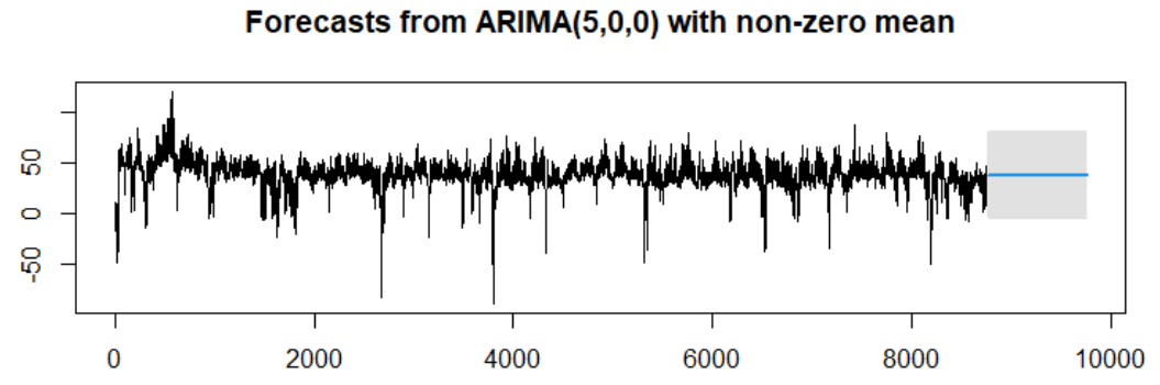
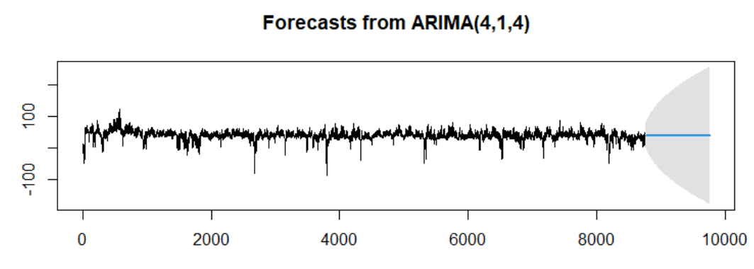
Follow the fpp3 text with these data. Notice some things:
- Better performance when limiting the training data to 200 points
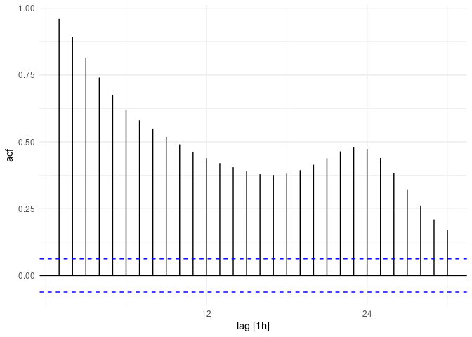
- Consistent weekly seasonality, but shifting daily
- Data require differencing
- Among the baseline model SNAIVE works best (tomorrow will be like yesterday)
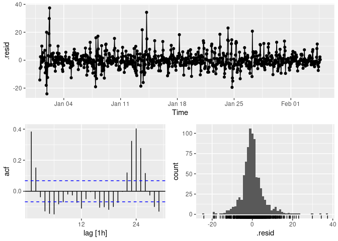
- An ARIMA model beats it slightly.
suppressPackageStartupMessages({
library(fpp3)
})
Time = seq(
from=as.POSIXct("2021-1-1 0:00", tz="UTC"),
to=as.POSIXct("2021-2-11 15:00", tz="UTC"),
by="hour")
DAT <- data.frame(Time, observed =
c(10.07, -4.08, -9.91, -7.41, -12.55, -17.25, -15.07, -4.93,
-6.33, -4.93, 0.45, 0.12, -0.02, 0, -0.03, 1.97, 9.06, 0.07,
-4.97, -6.98, -24.93, -4.87, -28.93, -33.57, -45.92, -48.29,
-44.99, -48.93, -29.91, -0.01, 37.43, 48.06, 50.74, 47.57, 43.94,
40.97, 44.95, 49.64, 53.67, 56.01, 56.95, 62.08, 62.11, 57.99,
55.64, 55.13, 50.76, 42.91, 45.22, 45.63, 44, 43.88, 45.92, 51.07,
52.77, 62.89, 60.03, 58.19, 62.99, 63.52, 64.67, 65.24, 67.76,
68.41, 69.55, 67.28, 69.46, 68.38, 61.72, 53.72, 49.98, 50.73,
47.11, 47.07, 46.94, 47, 46.91, 49.59, 55.32, 55.78, 55.52, 55.23,
53.58, 51.74, 51.6, 51.41, 51.69, 52.59, 54.66, 54.1, 51.89,
46.58, 45.43, 43.96, 31.41, 26.9, 25.12, 24.12, 22.04, 18.37,
22.09, 23.35, 28.76, 36.63, 40.46, 45.85, 49.8, 51.36, 51.74,
51.92, 53.22, 56.62, 56.92, 61.64, 59.44, 52.75, 51.9, 51.38,
49.96, 50.29, 47.72, 48.38, 48.02, 44.23, 47.17, 48.19, 49.11,
50.44, 53.4, 56.55, 60.02, 60.22, 55, 52.39, 51.57, 54.71, 63.43,
67.37, 67.2, 66.03, 55.36, 58.59, 53.7, 46.03, 47.98, 47.84,
46.11, 46.08, 47.62, 55.77, 68.61, 74.15, 74.93, 73.59, 71.23,
68.79, 66.75, 62.47, 53.25, 53.26, 53.42, 47.91, 42.05, 40.96,
32.04, 20.82, 1.84, 17.94, 20.91, 7.78, 14.33, 18.56, 18.57,
35.81, 43.87, 46.93, 43.88, 43.85, 46.74, 43.94, 43.21, 43.81,
45.6, 35.21, 45.64, 45.63, 37.94, 39.53, 35.97, 29.72, 22.55,
20.04, 7.24, 3.43, 10.04, 14.2, 25.41, 36.98, 43.89, 50.98, 50.3,
50.21, 45.8, 43.64, 43.49, 45.05, 49.95, 53.82, 55.94, 54.19,
54.19, 52.98, 51.68, 48.95, 47.63, 46.48, 49.08, 47.11, 48.8,
48.5, 49.8, 56.97, 72.6, 81.17, 81.79, 81.15, 80, 76.39, 75,
76.06, 75.4, 76.78, 83.45, 85.15, 78.16, 71.92, 67.43, 60.49,
54.45, 47.84, 46.58, 45.74, 43.81, 46.24, 46.46, 51.29, 60.53,
60.02, 62.92, 61.58, 60.6, 51.89, 50.8, 45.46, 42.2, 45, 51.51,
48.59, 49.2, 44.99, 44.93, 46.4, 43.46, 47.24, 45.88, 44.61,
42.9, 42.03, 39.33, 42.98, 41.23, 42.12, 45.1, 44.27, 44.18,
42.05, 38.61, 37.76, 33.03, 35.84, 44.24, 46.29, 40.05, 38.15,
30.26, 40.2, 30.89, 23.35, 12.4, 19.01, 23.51, 23.25, 20.01,
20.8, 22.14, 23.68, 25.05, 26.3, 30.81, 27.06, 8.5, -0.08, -0.01,
-0.27, 21.55, 24.04, 15.91, -0.02, -0.33, 3.04, -7.28, -3.14,
-12, -15.04, -11.09, -4.94, 1.59, 35.9, 51.22, 51.66, 46.09,
50.26, 44.49, 41.24, 38.91, 41.79, 49.63, 50.93, 51.25, 50.93,
50.52, 49.61, 44.3, 41.29, 37.26, 35.18, 35.82, 34.99, 34.56,
30.8, 33.41, 47.4, 53.73, 57.02, 58.38, 56.54, 55, 53.92, 53.31,
52.63, 52.12, 51, 53.91, 46.35, 42.73, 40.32, 39.93, 39.66, 32.04,
29.23, 29.26, 32.64, 32.41, 33.06, 33.22, 46.63, 53.8, 55.73,
53.83, 54.22, 54.92, 53.65, 52.69, 53.55, 53.72, 54.83, 54.01,
52.67, 50.92, 39.81, 39.29, 39.91, 30.77, 26.35, 25.23, 22.77,
24.02, 25.63, 28.06, 35.38, 46.04, 49.96, 50.56, 46.1, 46.02,
43.94, 46.64, 55, 55.9, 57.43, 58.72, 55.06, 53.85, 49.52, 42.35,
42.44, 41.11, 42.26, 40.91, 43.77, 45.05, 47.89, 49.79, 54.77,
73.08, 76.86, 74.32, 70.51, 69.02, 68.94, 65.27, 67.44, 68.14,
69, 75.04, 76.13, 72.46, 61.83, 59.24, 56.7, 53.16, 52.47, 53.18,
54.73, 51.15, 52.25, 50.93, 49.04, 50.56, 55.71, 56.62, 63.13,
57.33, 55.26, 54.38, 52.55, 55.41, 62.93, 67.15, 68.91, 57.37,
54.61, 52.32, 51.53, 49.8, 47.74, 47.01, 48.8, 48.9, 49.63, 49.53,
46.69, 46.76, 50.88, 52.38, 50.07, 49.33, 48.98, 47.4, 53.2,
55.39, 58.02, 66.68, 69.43, 69.75, 67.83, 57.37, 59.56, 52.07,
55.54, 53.02, 52.1, 51.31, 51.14, 53.23, 67.16, 79.62, 88.06,
86.01, 80.04, 75, 70.65, 71.56, 72.03, 76.49, 81.08, 88.35, 88.5,
79.93, 73.69, 68.34, 59.83, 54.93, 54.19, 54.05, 53.52, 51.97,
51.96, 52.03, 62.33, 73.91, 80.23, 76.6, 74.19, 70.06, 62.07,
58.45, 59.69, 65.09, 70.21, 78.8, 74.13, 64.46, 58.34, 55.38,
56.59, 53.72, 53.2, 53.92, 53.11, 51.19, 51.02, 55.05, 63.96,
82.55, 92.15, 93.65, 91.93, 88.07, 84.96, 83.99, 85.59, 86.87,
84.96, 90.01, 93.76, 90.54, 78.49, 68.93, 65.1, 59, 61.88, 59.08,
57.9, 56.37, 56.95, 61.53, 75.98, 99.07, 113.07, 111.23, 108.25,
103.69, 98.33, 92.63, 89.86, 90.45, 95.01, 106.82, 121.46, 102.06,
89.34, 74.43, 69.92, 63.79, 64.63, 60.64, 57.8, 55.44, 55.28,
58.98, 71.1, 84.48, 97, 93.64, 85, 78, 71.81, 69.87, 68.64, 65.58,
65.08, 70.87, 71.74, 58.51, 50.78, 51.12, 47.16, 42.9, 44.29,
42.61, 42.51, 41.96, 41.65, 40.72, 41.53, 42.36, 51.37, 56.28,
58.62, 59.18, 56.72, 57.44, 53.32, 52.8, 52.44, 55.95, 57.92,
53.78, 47.98, 44.99, 43.9, 37.75, 28.42, 24.48, 19.98, 18.13,
13.61, 15.34, 3.65, 24.47, 27.04, 32.97, 39.06, 44.05, 46.86,
42.97, 41.18, 40.5, 41.18, 47.25, 52.64, 52.96, 50.44, 47.74,
50.82, 44.81, 42.4, 40.97, 40.42, 37.8, 38.09, 41.83, 53.09,
64.04, 64.88, 62.2, 58.38, 55.92, 55.12, 51.36, 48.63, 47.34,
48.83, 60.83, 59.64, 54.37, 47.54, 45.69, 46.36, 43.91, 44.87,
48.07, 47.49, 44.59, 45.97, 46.46, 55.82, 67.67, 72.8, 70.63,
70.38, 67.51, 64.03, 63.84, 66.56, 66, 69.33, 71.45, 72.82, 69.81,
59.51, 55.74, 53.83, 49.34, 46.52, 46.36, 45.1, 42.85, 42.74,
46.34, 52.09, 64.99, 68.17, 66.76, 59.06, 53.03, 54.19, 49.7,
53.56, 49.37, 52.65, 60.49, 62.53, 59.28, 50.02, 51.01, 50.08,
46.86, 47.17, 45.47, 45.43, 46.82, 45.08, 48.7, 62.41, 71.7,
78.49, 69.08, 67.35, 67.94, 66.81, 66.22, 66.16, 66.16, 65.35,
66.68, 66.98, 65.4, 59.9, 52.84, 51.36, 46.72, 43.55, 45.47,
43.1, 41.1, 41.51, 45.76, 47.72, 54.04, 56.66, 55.93, 55.51,
56.9, 58.51, 64, 64.93, 64.55, 63.91, 67.71, 69.98, 67.34, 62.99,
55.32, 54.01, 50.92, 50.04, 47.07, 45.7, 43.14, 42.71, 42.6,
43.47, 47.68, 51.47, 55.79, 59.5, 59.15, 56.08, 50.33, 49.09,
48.6, 49.39, 56.86, 57.91, 54.59, 50.43, 48.48, 48.49, 46.06,
44.8, 41.29, 40.48, 39, 38.9, 38.47, 39.88, 40.97, 43.8, 47.05,
49.33, 51.11, 50.35, 47.09, 45.14, 44.4, 45.79, 51.94, 59.54,
57.94, 54.69, 51.94, 51.04, 46.42, 43.7, 41.37, 40.48, 39.21,
38.55, 40.71, 49.05, 60.67, 58.93, 55.47, 48.15, 43.46, 41.69,
40.47, 41.01, 43.37, 43.82, 49.06, 46.78, 42.08, 39.42, 38.75,
38.52, 32.51, 34.49, 36.71, 38.42, 39.39, 39.82, 41.72, 50.31,
61.52, 62.31, 62.31, 64.56, 62.85, 58.63, 57.81, 57.96, 58.04,
60.35, 63.06, 65.79, 62.63, 61.77, 53.38, 50.12, 46.98, 42.8,
41.63, 40.98, 40.4, 41.38, 42.31, 51.1, 57.59, 59.01, 53.34,
53.54, 53.32, 53.19, 52.81, 52.93, 54.3, 56.73, 60.27, 62.4,
59.62, 55.8, 50.49, 49.5, 46.18, 46.25, 45.21, 41.24, 38.05,
37, 39.04, 48.06, 53.29, 53.04, 51.98, 51.47, 46.38, 43.24, 42.32,
40.75, 41.63, 41.77, 51.37, 51.4, 45.75, 46.07, 41.47, 38.71,
33.68, 32.73, 33.24, 32.57, 31.16, 35.71, 38.99, 45.85, 56.33,
57.94, 54.91, 51.35, 50.66, 44.59, 39.51, 38.77, 42.31, 43.98,
49.61, 50.66, 46.04, 35.88, 33.96, 27.56, 24.47, 0.02, 0.08,
-4.09, -4, 0.06, 0.09, 0.05, 6.37, 12.08, 11.18, 10.64, 4.12,
0.05, -0.1, -2.05, 0.09, 9.64, 26.97, 36.17, 25.97, 16.96, 0.09,
12.91, 0.09, 22.88, 16.16, 16.02, 12.45, 10.19, 14.51, 7.01,
10.98, 20.62, 32.95, 36.75, 38.68, 32.5, 34, 31.2, 27.99, 32.61,
39.41, 49.19, 49.48, 43.1, 28.99, 34.37, 30.58, -0.01, -1.22,
-0.04, -3.54, -3.95, 5.65, 39.91, 49.04, 49.41, 44.99, 39.94,
38.73, 36.59, 38.54, 38.66, 38.86, 38.61)
)
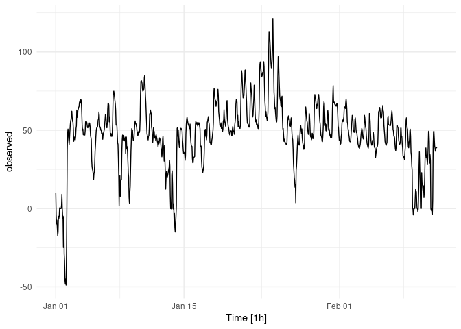
dat <- tsibble(DAT,index=Time)
autoplot(dat) + theme_minimal()
#> Plot variable not specified, automatically selected `.vars = observed`

dat %>%
features(observed, feature_set(pkgs="feasts")) %>%
t()
#> Warning: `n_flat_spots()` is deprecated as of feasts 0.1.5.
#> Please use `longest_flat_spot()` instead.
#> This warning is displayed once every 8 hours.
#> Call `lifecycle::last_warnings()` to see where this warning was generated.
#> [,1]
#> trend_strength 0.88495741
#> seasonal_strength_day 0.66506048
#> seasonal_peak_day 18.00000000
#> seasonal_trough_day 4.00000000
#> spikiness 0.00993752
#> linearity 40.49057987
#> curvature -302.36974156
#> stl_e_acf1 0.79002898
#> stl_e_acf10 1.10419120
#> acf1 0.96037775
#> acf10 4.92120104
#> diff1_acf1 0.34763257
#> diff1_acf10 0.22523960
#> diff2_acf1 -0.34315344
#> diff2_acf10 0.14589570
#> season_acf1 0.47364536
#> pacf5 1.07745209
#> diff1_pacf5 0.29758087
#> diff2_pacf5 0.48252887
#> season_pacf -0.21001083
#> zero_run_mean 1.00000000
#> nonzero_squared_cv 0.20238202
#> zero_start_prop 0.00000000
#> zero_end_prop 0.00000000
#> lambda_guerrero 1.37960539
#> kpss_stat 0.86876471
#> kpss_pvalue 0.01000000
#> pp_stat -5.49506838
#> pp_pvalue 0.01000000
#> ndiffs 1.00000000
#> nsdiffs 1.00000000
#> bp_stat 922.32541540
#> bp_pvalue 0.00000000
#> lb_stat 925.09516140
#> lb_pvalue 0.00000000
#> var_tiled_var 0.31164518
#> var_tiled_mean 0.65299865
#> shift_level_max 63.92541667
#> shift_level_index 31.00000000
#> shift_var_max 1803.47726444
#> shift_var_index 21.00000000
#> shift_kl_max 140.50454837
#> shift_kl_index 30.00000000
#> spectral_entropy 0.65228686
#> n_crossing_points 90.00000000
#> longest_flat_spot 27.00000000
#> coef_hurst 0.99958586
#> stat_arch_lm 0.86069565
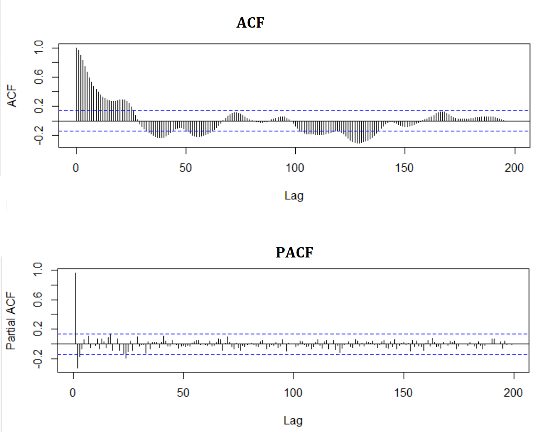
dat %>% ACF(observed) %>% autoplot() + theme_minimal()
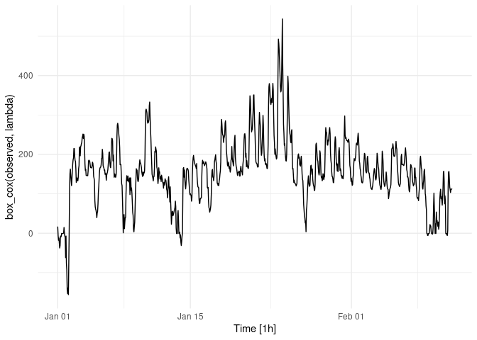
lambda <- dat %>%
  features(observed, features = guerrero) %>%
  pull(lambda_guerrero)

dat %>% autoplot(box_cox(observed, lambda)) + theme_minimal()
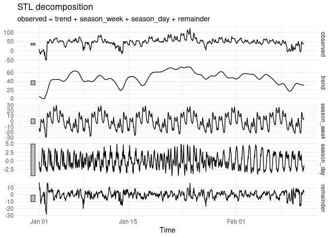
dcmp <- dat %>%
model(STL(observed))
components(dcmp)
#> # A dable: 1,000 x 8 [1h] <UTC>
#> # Key: .model [1]
#> # STL Decomposition: observed = trend + season_week + season_day + remainder
#> .model Time observed trend season_week season_day remainder
#> <chr> <dttm> <dbl> <dbl> <dbl> <dbl> <dbl>
#> 1 STL(o… 2021-01-01 00:00:00 10.1 5.05 -12.4 -0.228 17.6
#> 2 STL(o… 2021-01-01 01:00:00 -4.08 4.59 -18.0 -2.16 11.5
#> 3 STL(o… 2021-01-01 02:00:00 -9.91 4.13 -18.9 -1.97 6.84
#> 4 STL(o… 2021-01-01 03:00:00 -7.41 3.68 -18.0 -2.98 9.89
#> 5 STL(o… 2021-01-01 04:00:00 -12.6 3.22 -18.3 -2.01 4.54
#> 6 STL(o… 2021-01-01 05:00:00 -17.2 2.77 -9.21 -2.85 -7.95
#> 7 STL(o… 2021-01-01 06:00:00 -15.1 2.41 -1.19 -3.29 -13.0
#> 8 STL(o… 2021-01-01 07:00:00 -4.93 2.05 3.90 -2.09 -8.80
#> 9 STL(o… 2021-01-01 08:00:00 -6.33 1.70 2.21 -1.50 -8.73
#> 10 STL(o… 2021-01-01 09:00:00 -4.93 1.34 1.60 -0.464 -7.40
#> # … with 990 more rows, and 1 more variable: season_adjust <dbl>
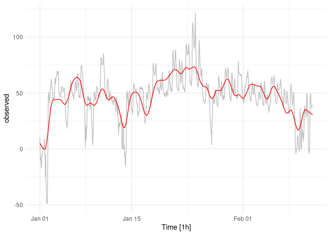
autoplot(dat, observed, color = "gray") +
autolayer(components(dcmp), trend, color = "red") +
theme_minimal()
components(dcmp) %>% autoplot() + theme_minimal()
# Break off held-out
past <- head(dat,832)
future <- tail(dat,24*7)
bench_fit <- past %>%
model(
Mean = MEAN(observed),
`Naïve` = NAIVE(observed),
Drift = NAIVE(observed ~ drift()),
`Seasonal Naïve` = SNAIVE(observed))
# Produce forecasts mid-February 2021
fc <- bench_fit %>% forecast(new_data = future)
fc %>% bench_fit <- past %>%
model(
Mean = MEAN(observed),
`Naïve` = NAIVE(observed),
Drift = NAIVE(observed ~ drift()),
`Seasonal Naïve` = SNAIVE(observed))
#> Error in fc %>% bench_fit <- past %>% model(Mean = MEAN(observed), Naïve = NAIVE(observed), : could not find function "%>%<-"
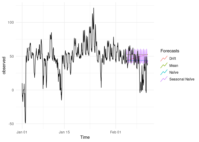
autoplot(past, level = NULL) +
autolayer(future, observed, color = "black") +
guides(colour = guide_legend(title = "Forecasts")) +
theme_minimal()
#> Plot variable not specified, automatically selected `.vars = observed`
#> Warning: Ignoring unknown parameters: level
accuracy(fc,future)
#> # A tibble: 4 x 9
#> .model .type ME RMSE MAE MPE MAPE MASE ACF1
#> <chr> <chr> <dbl> <dbl> <dbl> <dbl> <dbl> <dbl> <dbl>
#> 1 Drift Test -10.6 22.5 16.5 -666. 8844. NaN 0.942
#> 2 Mean Test -12.8 22.7 16.4 -816. 8919. NaN 0.936
#> 3 Naïve Test -7.13 20.0 14.6 -712. 7900. NaN 0.936
#> 4 Seasonal Naïve Test -11.0 20.7 14.4 -815. 7833. NaN 0.942
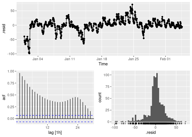
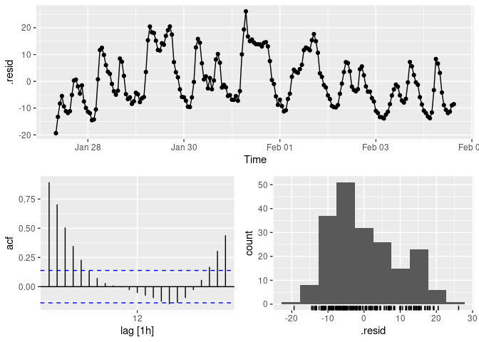
# Plot the diagnostics
past %>%
model(
Mean = MEAN(observed)) %>%
gg_tsresiduals()
past %>%
  model(`Naïve` = NAIVE(observed)) %>%
    gg_tsresiduals()
#> Warning: Removed 1 row(s) containing missing values (geom_path).
#> Warning: Removed 1 rows containing missing values (geom_point).
#> Warning: Removed 1 rows containing non-finite values (stat_bin).

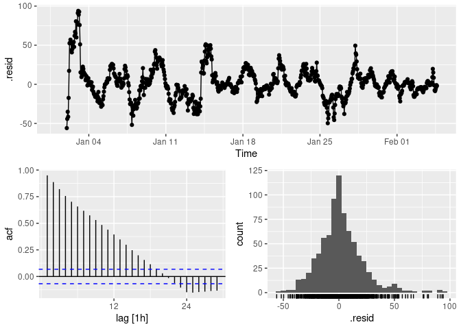
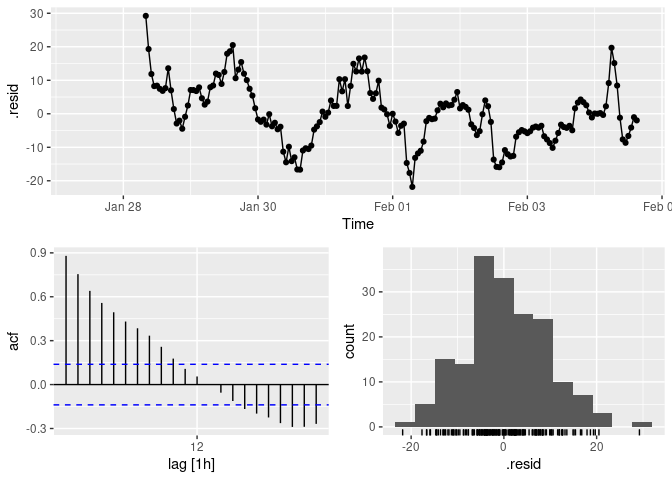
past %>%
  model(Drift = NAIVE(observed ~ drift())) %>%
  gg_tsresiduals()
#> Warning: Removed 1 row(s) containing missing values (geom_path).
#> Warning: Removed 1 rows containing missing values (geom_point).
#> Warning: Removed 1 rows containing non-finite values (stat_bin).
past %>%
  model(`Seasonal Naïve` = SNAIVE(observed)) %>%
  gg_tsresiduals()
#> Warning: Removed 24 row(s) containing missing values (geom_path).
#> Warning: Removed 24 rows containing missing values (geom_point).
#> Warning: Removed 24 rows containing non-finite values (stat_bin).
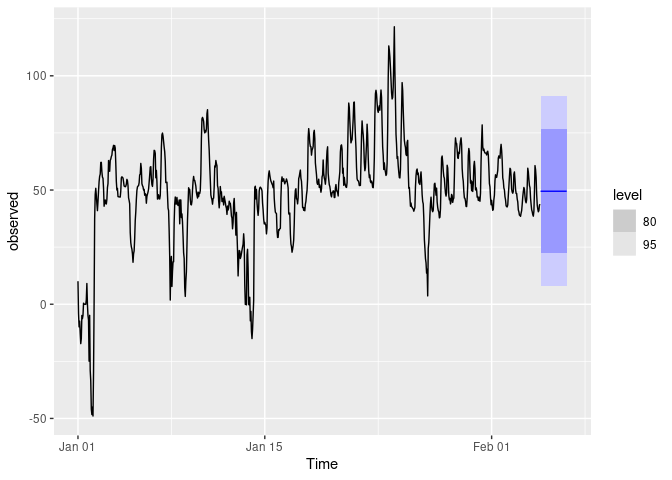
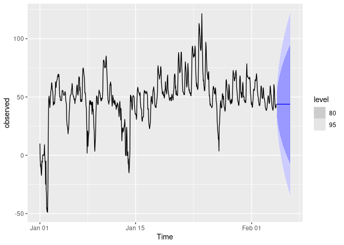
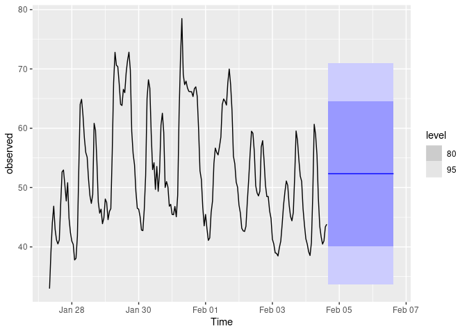
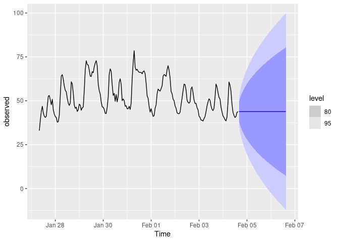
past %>%
  model(MEAN(observed)) %>%
  forecast(h = 48) %>%
  autoplot(past)
past %>%
  model(NAIVE(observed)) %>%
  forecast(h = 48) %>%
  autoplot(past)
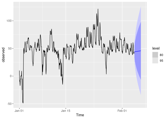
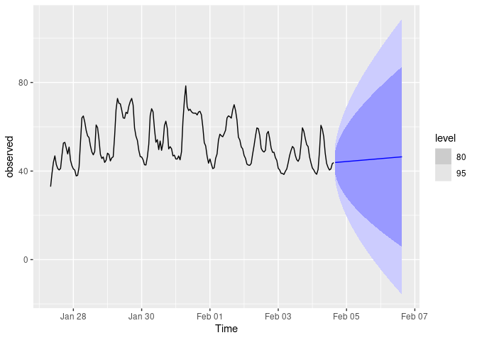
past %>%
  model(Drift = NAIVE(observed ~ drift())) %>%
  forecast(h = 48) %>%
  autoplot(past)
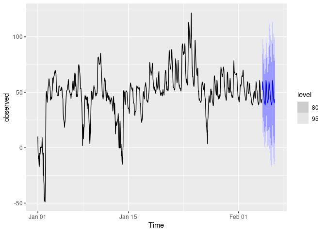
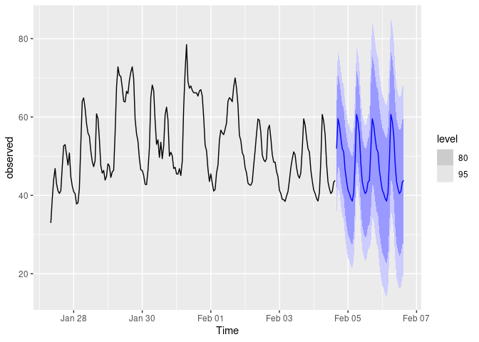
past %>%
  model(SNAIVE(observed)) %>%
  forecast(h = 48) %>%
  autoplot(past)
augment(bench_fit) %>% features(.innov, box_pierce, lag = 24, dof = 0)
#> # A tibble: 4 x 3
#> .model bp_stat bp_pvalue
#> <chr> <dbl> <dbl>
#> 1 Drift 501. 0
#> 2 Mean 5813. 0
#> 3 Naïve 501. 0
#> 4 Seasonal Naïve 4708. 0
short_past <- tail(past,200)
bench_fit2 <- short_past %>%
model(
Mean = MEAN(observed),
`Naïve` = NAIVE(observed),
Drift = NAIVE(observed ~ drift()),
`Seasonal Naïve` = SNAIVE(observed))
fc2 <- bench_fit2 %>% forecast(new_data = future)
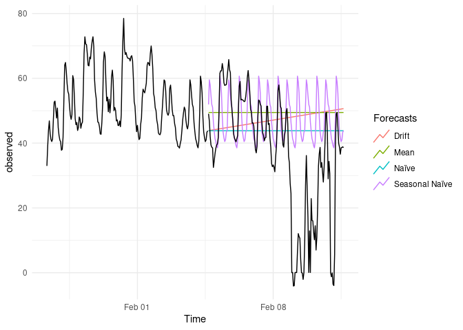
fc2 %>%
autoplot(past, level = NULL) +
autolayer(future, observed, color = "black") +
guides(colour = guide_legend(title = "Forecasts")) +
theme_minimal()
accuracy(fc2,future)
#> # A tibble: 4 x 9
#>   .model         .type     ME  RMSE   MAE   MPE  MAPE  MASE  ACF1
#>   <chr>          <chr>  <dbl> <dbl> <dbl> <dbl> <dbl> <dbl> <dbl>
#> 1 Drift          Test  -11.7   23.5  17.3 -650. 9168.   NaN 0.945
#> 2 Mean           Test  -15.6   24.4  18.0 -870. 9441.   NaN 0.936
#> 3 Naïve          Test   -7.13  20.0  14.6 -712. 7900.   NaN 0.936
#> 4 Seasonal Naïve Test  -11.0   20.7  14.4 -815. 7833.   NaN 0.942

short_past %>%
  model(
  Mean = MEAN(observed)) %>%
  gg_tsresiduals()
short_past %>%
  model(`Naïve` = NAIVE(observed)) %>%
  gg_tsresiduals()
#> Warning: Removed 1 row(s) containing missing values (geom_path).
#> Warning: Removed 1 rows containing missing values (geom_point).
#> Warning: Removed 1 rows containing non-finite values (stat_bin).

short_past %>%
  model(Drift = NAIVE(observed ~ drift())) %>%
  gg_tsresiduals()
#> Warning: Removed 1 row(s) containing missing values (geom_path).
#> Warning: Removed 1 rows containing missing values (geom_point).
#> Warning: Removed 1 rows containing non-finite values (stat_bin).
short_past %>%
  model(`Seasonal Naïve` = SNAIVE(observed)) %>%
  gg_tsresiduals()
#> Warning: Removed 24 row(s) containing missing values (geom_path).
#> Warning: Removed 24 rows containing missing values (geom_point).
#> Warning: Removed 24 rows containing non-finite values (stat_bin).
short_past %>%
  model(MEAN(observed)) %>%
  forecast(h = 48) %>%
  autoplot(short_past)
short_past %>%
  model(NAIVE(observed)) %>%
  forecast(h = 48) %>%
  autoplot(short_past)
short_past %>%
  model(Drift = NAIVE(observed ~ drift())) %>%
  forecast(h = 48) %>%
  autoplot(short_past)
short_past %>%
  model(SNAIVE(observed)) %>%
  forecast(h = 48) %>%
  autoplot(short_past)
short_past %>%
  features(observed, unitroot_kpss)
#> # A tibble: 1 x 2
#>   kpss_stat kpss_pvalue
#>       <dbl>       <dbl>
#> 1     0.381      0.0856

short_past %>%
  mutate(diff_observed = difference(observed)) %>%
  features(diff_observed, unitroot_kpss)
#> # A tibble: 1 x 2
#>   kpss_stat kpss_pvalue
#>       <dbl>       <dbl>
#> 1    0.0564         0.1

short_past %>%
  mutate(diff_observed = difference(observed)) -> d

bench_fitd <- past %>%
  model(
    Mean = MEAN(observed),
    `Naïve` = NAIVE(observed),
    Drift = NAIVE(observed ~ drift()),
    `Seasonal Naïve` = SNAIVE(observed))

fcd <- bench_fitd %>% forecast(new_data = future)

fcd %>%
  autoplot(d, level = NULL) +
  autolayer(future, observed, color = "black") +
  guides(colour = guide_legend(title = "Forecasts")) +
  theme_minimal()
accuracy(fcd,future)
#> # A tibble: 4 x 9
#>   .model         .type     ME  RMSE   MAE   MPE  MAPE  MASE  ACF1
#>   <chr>          <chr>  <dbl> <dbl> <dbl> <dbl> <dbl> <dbl> <dbl>
#> 1 Drift          Test  -10.6   22.5  16.5 -666. 8844.   NaN 0.942
#> 2 Mean           Test  -12.8   22.7  16.4 -816. 8919.   NaN 0.936
#> 3 Naïve          Test   -7.13  20.0  14.6 -712. 7900.   NaN 0.936
#> 4 Seasonal Naïve Test  -11.0   20.7  14.4 -815. 7833.   NaN 0.942

# Plot the diagnostics

d %>%
  model(Mean = MEAN(observed)) %>%
  gg_tsresiduals()
d %>%
  model(`Naïve` = NAIVE(observed)) %>%
  gg_tsresiduals()
#> Warning: Removed 1 row(s) containing missing values (geom_path).
#> Warning: Removed 1 rows containing missing values (geom_point).
#> Warning: Removed 1 rows containing non-finite values (stat_bin).
d %>%
  model(Drift = NAIVE(observed ~ drift())) %>%
  gg_tsresiduals()
#> Warning: Removed 1 row(s) containing missing values (geom_path).
#> Warning: Removed 1 rows containing missing values (geom_point).
#> Warning: Removed 1 rows containing non-finite values (stat_bin).
d %>%
  model(`Seasonal Naïve` = SNAIVE(observed)) %>%
  gg_tsresiduals()
#> Warning: Removed 24 row(s) containing missing values (geom_path).
#> Warning: Removed 24 rows containing missing values (geom_point).
#> Warning: Removed 24 rows containing non-finite values (stat_bin).
d %>%
  model(MEAN(observed)) %>%
  forecast(h = 48) %>%
  autoplot(d)
d %>%
  model(NAIVE(observed)) %>%
  forecast(h = 48) %>%
  autoplot(d)
d %>%
  model(Drift = NAIVE(observed ~ drift())) %>%
  forecast(h = 48) %>%
  autoplot(d)
d %>%
  model(SNAIVE(observed)) %>%
  forecast(h = 48) %>%
  autoplot(d)
augment(bench_fit) %>% features(.innov, box_pierce, lag = 24, dof = 0)
#> # A tibble: 4 x 3
#> .model bp_stat bp_pvalue
#> <chr> <dbl> <dbl>
#> 1 Drift 501. 0
#> 2 Mean 5813. 0
#> 3 Naïve 501. 0
#> 4 Seasonal Naïve 4708. 0
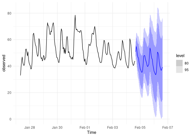
d %>% model(ARIMA(observed)) -> afit
d %>%
model(ARIMA(observed)) %>%
forecast(h = 48) %>%
autoplot(d) + theme_minimal()
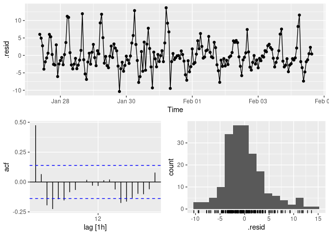
d %>%
  model(ARIMA(observed)) %>%
  gg_tsresiduals()
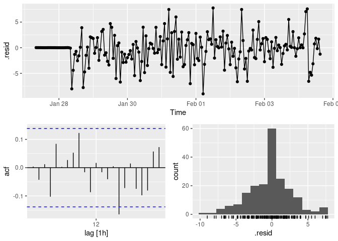
augment(afit) %>%
  features(.innov, ljung_box, lag = 24, dof = 1)
#> # A tibble: 1 x 3
#>   .model          lb_stat lb_pvalue
#>   <chr>             <dbl>     <dbl>
#> 1 ARIMA(observed)    26.9     0.262

fca <- afit %>% forecast(new_data = future)

accuracy(fca,future)
#> # A tibble: 1 x 9
#>   .model          .type     ME  RMSE   MAE   MPE  MAPE  MASE  ACF1
#>   <chr>           <chr>  <dbl> <dbl> <dbl> <dbl> <dbl> <dbl> <dbl>
#> 1 ARIMA(observed) Test  -0.512  14.9  12.0 -866. 5291.   NaN 0.926
Created on 2021-01-08 by the reprex package (v0.3.0.9001)