Here's what I meant. Can you specify the commented out fit2 at the bottom and post back the reprex?
suppressPackageStartupMessages({
library(fpp3)
library(patchwork)
})
Time <- seq(
from = as.POSIXct("2021-1-1 0:00", tz = "UTC"),
to = as.POSIXct("2021-2-11 15:00", tz = "UTC"),
by = "hour"
)
DAT <- data.frame(Time,
observed =
c(
10.07, -4.08, -9.91, -7.41, -12.55, -17.25, -15.07, -4.93,
-6.33, -4.93, 0.45, 0.12, -0.02, 0, -0.03, 1.97, 9.06, 0.07,
-4.97, -6.98, -24.93, -4.87, -28.93, -33.57, -45.92, -48.29,
-44.99, -48.93, -29.91, -0.01, 37.43, 48.06, 50.74, 47.57, 43.94,
40.97, 44.95, 49.64, 53.67, 56.01, 56.95, 62.08, 62.11, 57.99,
55.64, 55.13, 50.76, 42.91, 45.22, 45.63, 44, 43.88, 45.92, 51.07,
52.77, 62.89, 60.03, 58.19, 62.99, 63.52, 64.67, 65.24, 67.76,
68.41, 69.55, 67.28, 69.46, 68.38, 61.72, 53.72, 49.98, 50.73,
47.11, 47.07, 46.94, 47, 46.91, 49.59, 55.32, 55.78, 55.52, 55.23,
53.58, 51.74, 51.6, 51.41, 51.69, 52.59, 54.66, 54.1, 51.89,
46.58, 45.43, 43.96, 31.41, 26.9, 25.12, 24.12, 22.04, 18.37,
22.09, 23.35, 28.76, 36.63, 40.46, 45.85, 49.8, 51.36, 51.74,
51.92, 53.22, 56.62, 56.92, 61.64, 59.44, 52.75, 51.9, 51.38,
49.96, 50.29, 47.72, 48.38, 48.02, 44.23, 47.17, 48.19, 49.11,
50.44, 53.4, 56.55, 60.02, 60.22, 55, 52.39, 51.57, 54.71, 63.43,
67.37, 67.2, 66.03, 55.36, 58.59, 53.7, 46.03, 47.98, 47.84,
46.11, 46.08, 47.62, 55.77, 68.61, 74.15, 74.93, 73.59, 71.23,
68.79, 66.75, 62.47, 53.25, 53.26, 53.42, 47.91, 42.05, 40.96,
32.04, 20.82, 1.84, 17.94, 20.91, 7.78, 14.33, 18.56, 18.57,
35.81, 43.87, 46.93, 43.88, 43.85, 46.74, 43.94, 43.21, 43.81,
45.6, 35.21, 45.64, 45.63, 37.94, 39.53, 35.97, 29.72, 22.55,
20.04, 7.24, 3.43, 10.04, 14.2, 25.41, 36.98, 43.89, 50.98, 50.3,
50.21, 45.8, 43.64, 43.49, 45.05, 49.95, 53.82, 55.94, 54.19,
54.19, 52.98, 51.68, 48.95, 47.63, 46.48, 49.08, 47.11, 48.8,
48.5, 49.8, 56.97, 72.6, 81.17, 81.79, 81.15, 80, 76.39, 75,
76.06, 75.4, 76.78, 83.45, 85.15, 78.16, 71.92, 67.43, 60.49,
54.45, 47.84, 46.58, 45.74, 43.81, 46.24, 46.46, 51.29, 60.53,
60.02, 62.92, 61.58, 60.6, 51.89, 50.8, 45.46, 42.2, 45, 51.51,
48.59, 49.2, 44.99, 44.93, 46.4, 43.46, 47.24, 45.88, 44.61,
42.9, 42.03, 39.33, 42.98, 41.23, 42.12, 45.1, 44.27, 44.18,
42.05, 38.61, 37.76, 33.03, 35.84, 44.24, 46.29, 40.05, 38.15,
30.26, 40.2, 30.89, 23.35, 12.4, 19.01, 23.51, 23.25, 20.01,
20.8, 22.14, 23.68, 25.05, 26.3, 30.81, 27.06, 8.5, -0.08, -0.01,
-0.27, 21.55, 24.04, 15.91, -0.02, -0.33, 3.04, -7.28, -3.14,
-12, -15.04, -11.09, -4.94, 1.59, 35.9, 51.22, 51.66, 46.09,
50.26, 44.49, 41.24, 38.91, 41.79, 49.63, 50.93, 51.25, 50.93,
50.52, 49.61, 44.3, 41.29, 37.26, 35.18, 35.82, 34.99, 34.56,
30.8, 33.41, 47.4, 53.73, 57.02, 58.38, 56.54, 55, 53.92, 53.31,
52.63, 52.12, 51, 53.91, 46.35, 42.73, 40.32, 39.93, 39.66, 32.04,
29.23, 29.26, 32.64, 32.41, 33.06, 33.22, 46.63, 53.8, 55.73,
53.83, 54.22, 54.92, 53.65, 52.69, 53.55, 53.72, 54.83, 54.01,
52.67, 50.92, 39.81, 39.29, 39.91, 30.77, 26.35, 25.23, 22.77,
24.02, 25.63, 28.06, 35.38, 46.04, 49.96, 50.56, 46.1, 46.02,
43.94, 46.64, 55, 55.9, 57.43, 58.72, 55.06, 53.85, 49.52, 42.35,
42.44, 41.11, 42.26, 40.91, 43.77, 45.05, 47.89, 49.79, 54.77,
73.08, 76.86, 74.32, 70.51, 69.02, 68.94, 65.27, 67.44, 68.14,
69, 75.04, 76.13, 72.46, 61.83, 59.24, 56.7, 53.16, 52.47, 53.18,
54.73, 51.15, 52.25, 50.93, 49.04, 50.56, 55.71, 56.62, 63.13,
57.33, 55.26, 54.38, 52.55, 55.41, 62.93, 67.15, 68.91, 57.37,
54.61, 52.32, 51.53, 49.8, 47.74, 47.01, 48.8, 48.9, 49.63, 49.53,
46.69, 46.76, 50.88, 52.38, 50.07, 49.33, 48.98, 47.4, 53.2,
55.39, 58.02, 66.68, 69.43, 69.75, 67.83, 57.37, 59.56, 52.07,
55.54, 53.02, 52.1, 51.31, 51.14, 53.23, 67.16, 79.62, 88.06,
86.01, 80.04, 75, 70.65, 71.56, 72.03, 76.49, 81.08, 88.35, 88.5,
79.93, 73.69, 68.34, 59.83, 54.93, 54.19, 54.05, 53.52, 51.97,
51.96, 52.03, 62.33, 73.91, 80.23, 76.6, 74.19, 70.06, 62.07,
58.45, 59.69, 65.09, 70.21, 78.8, 74.13, 64.46, 58.34, 55.38,
56.59, 53.72, 53.2, 53.92, 53.11, 51.19, 51.02, 55.05, 63.96,
82.55, 92.15, 93.65, 91.93, 88.07, 84.96, 83.99, 85.59, 86.87,
84.96, 90.01, 93.76, 90.54, 78.49, 68.93, 65.1, 59, 61.88, 59.08,
57.9, 56.37, 56.95, 61.53, 75.98, 99.07, 113.07, 111.23, 108.25,
103.69, 98.33, 92.63, 89.86, 90.45, 95.01, 106.82, 121.46, 102.06,
89.34, 74.43, 69.92, 63.79, 64.63, 60.64, 57.8, 55.44, 55.28,
58.98, 71.1, 84.48, 97, 93.64, 85, 78, 71.81, 69.87, 68.64, 65.58,
65.08, 70.87, 71.74, 58.51, 50.78, 51.12, 47.16, 42.9, 44.29,
42.61, 42.51, 41.96, 41.65, 40.72, 41.53, 42.36, 51.37, 56.28,
58.62, 59.18, 56.72, 57.44, 53.32, 52.8, 52.44, 55.95, 57.92,
53.78, 47.98, 44.99, 43.9, 37.75, 28.42, 24.48, 19.98, 18.13,
13.61, 15.34, 3.65, 24.47, 27.04, 32.97, 39.06, 44.05, 46.86,
42.97, 41.18, 40.5, 41.18, 47.25, 52.64, 52.96, 50.44, 47.74,
50.82, 44.81, 42.4, 40.97, 40.42, 37.8, 38.09, 41.83, 53.09,
64.04, 64.88, 62.2, 58.38, 55.92, 55.12, 51.36, 48.63, 47.34,
48.83, 60.83, 59.64, 54.37, 47.54, 45.69, 46.36, 43.91, 44.87,
48.07, 47.49, 44.59, 45.97, 46.46, 55.82, 67.67, 72.8, 70.63,
70.38, 67.51, 64.03, 63.84, 66.56, 66, 69.33, 71.45, 72.82, 69.81,
59.51, 55.74, 53.83, 49.34, 46.52, 46.36, 45.1, 42.85, 42.74,
46.34, 52.09, 64.99, 68.17, 66.76, 59.06, 53.03, 54.19, 49.7,
53.56, 49.37, 52.65, 60.49, 62.53, 59.28, 50.02, 51.01, 50.08,
46.86, 47.17, 45.47, 45.43, 46.82, 45.08, 48.7, 62.41, 71.7,
78.49, 69.08, 67.35, 67.94, 66.81, 66.22, 66.16, 66.16, 65.35,
66.68, 66.98, 65.4, 59.9, 52.84, 51.36, 46.72, 43.55, 45.47,
43.1, 41.1, 41.51, 45.76, 47.72, 54.04, 56.66, 55.93, 55.51,
56.9, 58.51, 64, 64.93, 64.55, 63.91, 67.71, 69.98, 67.34, 62.99,
55.32, 54.01, 50.92, 50.04, 47.07, 45.7, 43.14, 42.71, 42.6,
43.47, 47.68, 51.47, 55.79, 59.5, 59.15, 56.08, 50.33, 49.09,
48.6, 49.39, 56.86, 57.91, 54.59, 50.43, 48.48, 48.49, 46.06,
44.8, 41.29, 40.48, 39, 38.9, 38.47, 39.88, 40.97, 43.8, 47.05,
49.33, 51.11, 50.35, 47.09, 45.14, 44.4, 45.79, 51.94, 59.54,
57.94, 54.69, 51.94, 51.04, 46.42, 43.7, 41.37, 40.48, 39.21,
38.55, 40.71, 49.05, 60.67, 58.93, 55.47, 48.15, 43.46, 41.69,
40.47, 41.01, 43.37, 43.82, 49.06, 46.78, 42.08, 39.42, 38.75,
38.52, 32.51, 34.49, 36.71, 38.42, 39.39, 39.82, 41.72, 50.31,
61.52, 62.31, 62.31, 64.56, 62.85, 58.63, 57.81, 57.96, 58.04,
60.35, 63.06, 65.79, 62.63, 61.77, 53.38, 50.12, 46.98, 42.8,
41.63, 40.98, 40.4, 41.38, 42.31, 51.1, 57.59, 59.01, 53.34,
53.54, 53.32, 53.19, 52.81, 52.93, 54.3, 56.73, 60.27, 62.4,
59.62, 55.8, 50.49, 49.5, 46.18, 46.25, 45.21, 41.24, 38.05,
37, 39.04, 48.06, 53.29, 53.04, 51.98, 51.47, 46.38, 43.24, 42.32,
40.75, 41.63, 41.77, 51.37, 51.4, 45.75, 46.07, 41.47, 38.71,
33.68, 32.73, 33.24, 32.57, 31.16, 35.71, 38.99, 45.85, 56.33,
57.94, 54.91, 51.35, 50.66, 44.59, 39.51, 38.77, 42.31, 43.98,
49.61, 50.66, 46.04, 35.88, 33.96, 27.56, 24.47, 0.02, 0.08,
-4.09, -4, 0.06, 0.09, 0.05, 6.37, 12.08, 11.18, 10.64, 4.12,
0.05, -0.1, -2.05, 0.09, 9.64, 26.97, 36.17, 25.97, 16.96, 0.09,
12.91, 0.09, 22.88, 16.16, 16.02, 12.45, 10.19, 14.51, 7.01,
10.98, 20.62, 32.95, 36.75, 38.68, 32.5, 34, 31.2, 27.99, 32.61,
39.41, 49.19, 49.48, 43.1, 28.99, 34.37, 30.58, -0.01, -1.22,
-0.04, -3.54, -3.95, 5.65, 39.91, 49.04, 49.41, 44.99, 39.94,
38.73, 36.59, 38.54, 38.66, 38.86, 38.61
)
)
dat <- tsibble(DAT, index = Time)
past <- dat[1:200,]
future <- anti_join(dat,past)
#> Joining, by = c("Time", "observed")
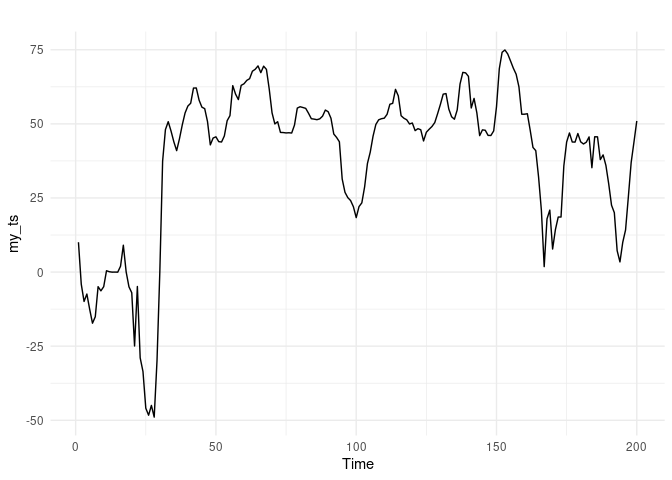
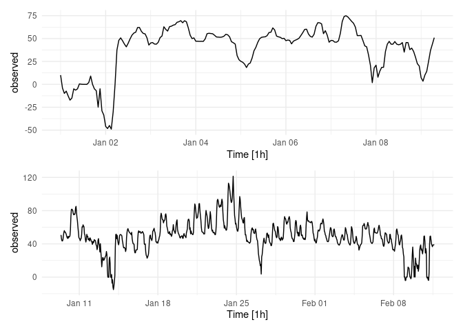
# always start with looking at the data
(autoplot(past) + theme_minimal()) / (autoplot(future) + theme_minimal())
#> Plot variable not specified, automatically selected `.vars = observed`
#> Plot variable not specified, automatically selected `.vars = observed`
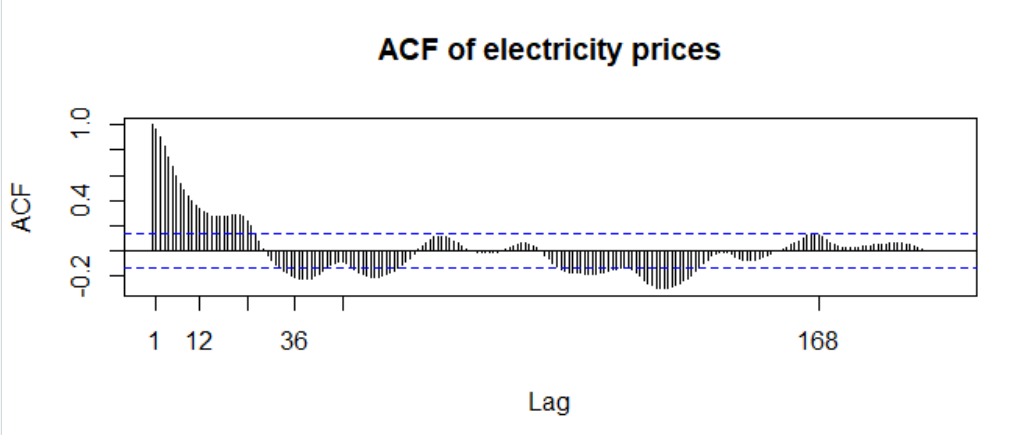
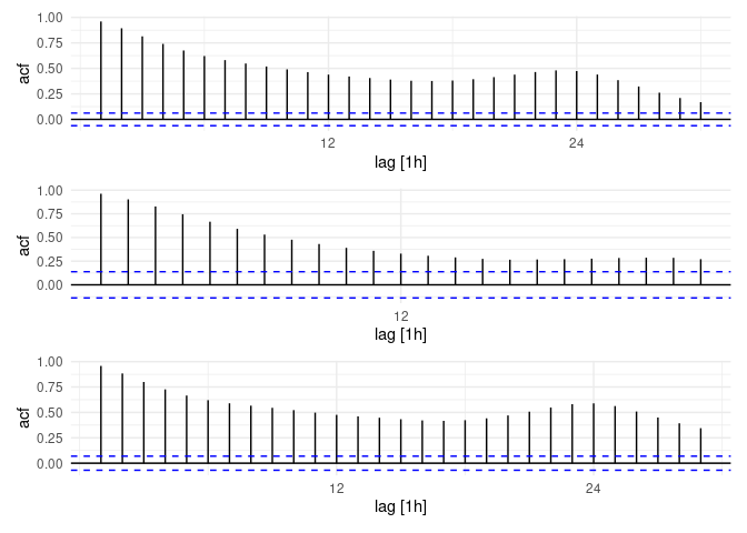
(dat %>% ACF(observed) %>% autoplot() + theme_minimal())   /
(past %>% ACF(observed) %>% autoplot() + theme_minimal())  /
(future %>% ACF(observed) %>% autoplot() + theme_minimal())
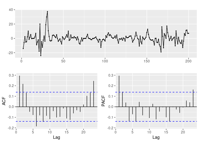
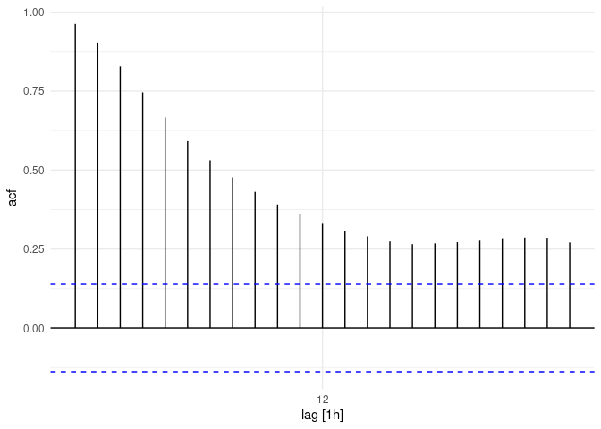
past %>%
  mutate(diffed = difference(observed)) %>%
  ACF() %>%
  autoplot() + theme_minimal()
#> Response variable not specified, automatically selected `var = observed`
past %>%
  mutate(diffed = difference(observed)) %>%
  PACF() %>%
  autoplot() + theme_minimal()
#> Response variable not specified, automatically selected `var = observed`
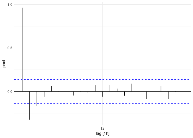
# ACF is sinusoidally declining and PACF has no peak after lag 1 suggests ARIMA(p,d,0) = 1,1,0
#
#Calculate auto ARIMA based on the first 200 entries (hours)
fit <- past %>%
model(auto = ARIMA(observed))
# unitroot test for stationarity
past %>%
features(observed, unitroot_kpss)
#> # A tibble: 1 x 2
#> kpss_stat kpss_pvalue
#> <dbl> <dbl>
#> 1 0.884 0.01
# test differenced
fit <- past %>%
model(auto = ARIMA(difference(observed)))
#> Error: No supported inverse for the `difference` transformation.
fit %>% report()
#> Series: observed
#> Model: ARIMA(1,1,1)(2,0,0)[24]
#>
#> Coefficients:
#> ar1 ma1 sar1 sar2
#> -0.8038 0.9197 0.1483 0.2914
#> s.e. 0.1112 0.0763 0.0750 0.1046
#>
#> sigma^2 estimated as 41.4: log likelihood=-653.57
#> AIC=1317.15 AICc=1317.46 BIC=1333.62
past %>%
mutate(diffed = difference(observed)) %>%
features(diffed, unitroot_kpss)
#> # A tibble: 1 x 2
#> kpss_stat kpss_pvalue
#> <dbl> <dbl>
#> 1 0.0401 0.1
# confirmation
past %>%
features(observed, unitroot_ndiffs)
#> # A tibble: 1 x 1
#> ndiffs
#> <int>
#> 1 1
# Portmanteau confirmation
augment(fit) %>%
features(.innov, ljung_box, dof = 1, lag = 12)
#> # A tibble: 1 x 3
#> .model lb_stat lb_pvalue
#> <chr> <dbl> <dbl>
#> 1 auto 19.6 0.0515
# no seasonal differencing
past %>% features(observed, unitroot_nsdiffs)
#> # A tibble: 1 x 1
#> nsdiffs
#> <int>
#> 1 0
# near zero mean, fit is not biased
mean(augment(fit)$.resid)
#> [1] 0.09024311
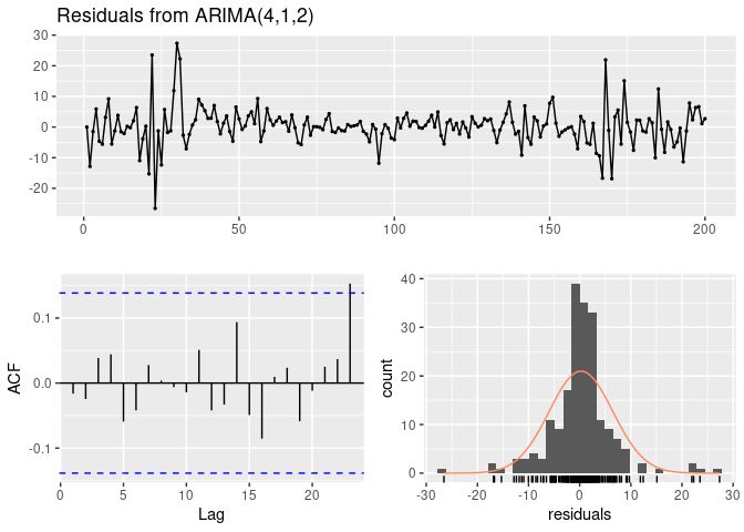
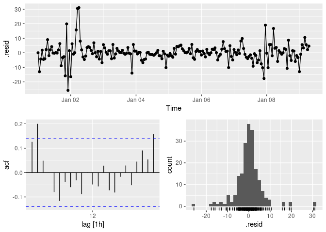
# lags at 2 and 23, approx normally distributed residuals
fit %>% gg_tsresiduals()
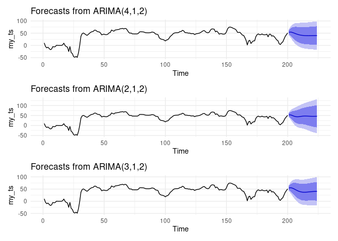
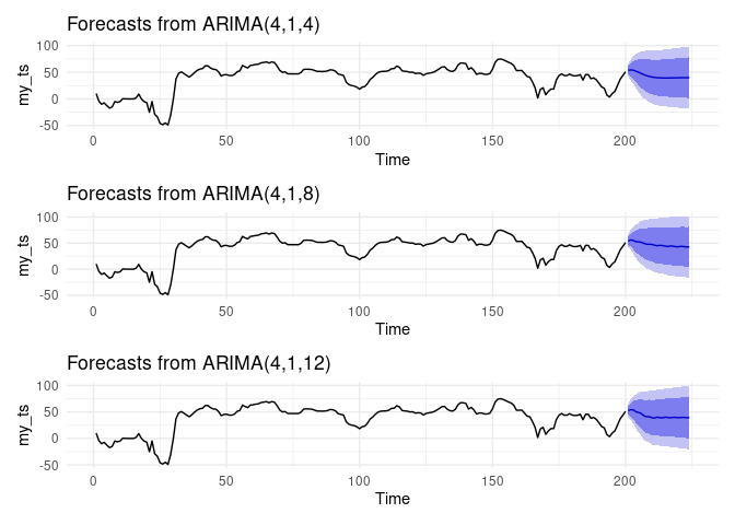
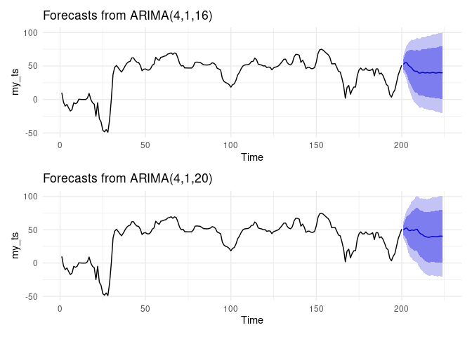
fc <- fit %>% forecast(new_data = future)
autoplot(fc) + theme_minimal()
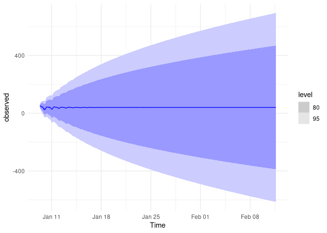
accuracy(fc,future)
#> # A tibble: 1 x 10
#>   .model .type    ME  RMSE   MAE   MPE  MAPE  MASE RMSSE  ACF1
#>   <chr>  <chr> <dbl> <dbl> <dbl> <dbl> <dbl> <dbl> <dbl> <dbl>
#> 1 auto   Test   9.47  21.4  16.5  738. 2416.   NaN   NaN 0.958

# fit2 <- past %>%
#   model(ar3120 = ARIMA(observed ~ 0 + pdq(3,1,20))) %>%
#   report()