Hello,
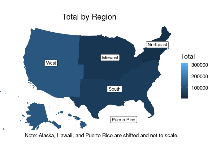
I'm trying to reproduce the following map in R:
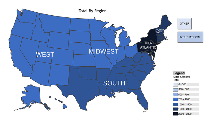
I got some help. Unfortunately, I'm running into two other issues:
-
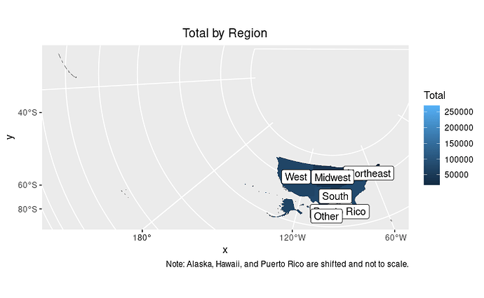
[Resolved] There is a lot of white space on the map. I would like to zoom into the main USA map. The tigris::shift_geometry() partially solved the problem by pulling Alaska, Hawaii, and Puerto Rico closer.
-
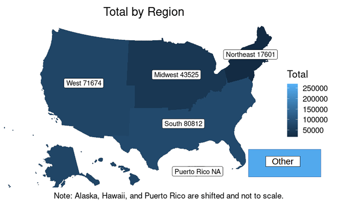
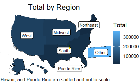
[Not Resolved] I need some way to include totals for regions outside of the USA. In the example map, the OTHER block serves to visualize the combined total for regions outside the USA. I tried to calculate the total for all non-US regions and combine the result with the US regions data.
Here is my attempt:
options(scipen = 999)
library(tidyverse)
library(tigris)
#> To enable
#> caching of data, set `options(tigris_use_cache = TRUE)` in your R script or .Rprofile.
library(sf)
#> Linking to GEOS 3.8.0, GDAL 3.0.4, PROJ 6.3.1
library(forcats)
library(ggrepel)
library(tidygeocoder)
library(knitr)
# Generate Data
data <- tibble::tribble(
~lon, ~lat,
-98.133208, 11.4326077,
-89.552784, 11.634501,
-62.2766186, 44.5090949,
-65.3279894, 33.1067754,
-67.7095365, 44.6294348,
-96.552784, 35.634501,
-97.3279093, 29.7724417,
-82.6363869, 28.2949194,
-80.2061931, 46.0133808,
-72.014118, 32.4681642,
-76.2531465, 47.3666368,
-82.1650991, 46.7758541,
-5.696645, 11.945587,
-112.707349, 38.5205043,
-63.0884036, 52.3930959,
-87.128901, 39.1242719,
-65.1626756, 31.3463503,
-94.3254958, 40.3274999,
-98.56121, 42.5770056,
-115.4429944, 46.1502862,
-117.7901088, 30.6913751,
-63.7389596, 54.6584068,
-109.1147095, 24.2156978,
-119.8340735, 22.6832497,
-117.8780275, 37.7311394,
-67.1763467, 38.5861576,
-96.4427769, 25.14644,
-78.0814292, 15.5386936,
-74.4185584, 34.5834425,
-77.4185584, 36.5834425,
-79.4185584, 37.5834425,
-63.121085, 33.9241038,
-88.121085, 41.9241038,
-112.7260713, 40.836309,
-90.552784, 30.634501,
-109.552784, 12.634501,
-73.9224329, 48.6153549
)
data <-
data %>% sample_n(100, replace = TRUE) %>%
mutate(
total = round( runif(nrow(.), min = 100, max = 10000), digits = 0) ,
lon = lon + round( runif(nrow(.), min = -10, max = 10), digits = 0),
lat = lat + round( runif(nrow(.), min = -10, max = 10), digits = 0)
)
data <- data %>%
reverse_geocode(
lat = lat,
long = lon,
method = 'arcgis',
full_results = TRUE,
return_input = TRUE,
return_coords = FALSE
)
data <- data %>% mutate(country = if_else(CountryCode == "USA", "USA", "Other"), state = if_else(CountryCode == "USA", Region, "International"))
# Download state data and filter states
sts <- states(cb = FALSE, resolution = "20m") %>%
shift_geometry()
#> | | | 0% | | | 1% | |= | 1% | |= | 2% | |== | 2% | |== | 3% | |=== | 4% | |=== | 5% | |==== | 6% | |======= | 9% | |======= | 10% | |======== | 11% | |======== | 12% | |========= | 12% | |========= | 13% | |========== | 15% | |=========== | 16% | |============ | 17% | |============= | 18% | |============= | 19% | |============== | 20% | |=============== | 21% | |================ | 23% | |================ | 24% | |================== | 26% | |=================== | 27% | |==================== | 29% | |===================== | 30% | |====================== | 32% | |======================= | 33% | |======================== | 34% | |======================== | 35% | |========================= | 35% | |========================== | 36% | |=========================== | 39% | |============================== | 42% | |============================== | 43% | |=============================== | 44% | |=============================== | 45% | |================================ | 46% | |================================== | 48% | |=================================== | 50% | |==================================== | 51% | |==================================== | 52% | |===================================== | 53% | |======================================= | 56% | |======================================== | 57% | |========================================= | 59% | |========================================== | 60% | |========================================== | 61% | |=========================================== | 61% | |=========================================== | 62% | |============================================ | 62% | |============================================ | 63% | |============================================= | 64% | |============================================== | 66% | |=============================================== | 67% | |================================================ | 68% | |================================================ | 69% | |================================================= | 70% | |================================================= | 71% | |================================================== | 71% | |=================================================== | 73% | |==================================================== | 74% | |==================================================== | 75% | |===================================================== | 75% | |====================================================== | 77% | |====================================================== | 78% | |======================================================= | 78% | |======================================================= | 79% | |======================================================== | 79% | |========================================================= | 81% | |========================================================= | 82% | |========================================================== | 83% | |========================================================== | 84% | |=========================================================== | 84% | |=========================================================== | 85% | |============================================================ | 85% | |============================================================ | 86% | |============================================================= | 86% | |============================================================= | 87% | |============================================================= | 88% | |============================================================== | 88% | |============================================================== | 89% | |=============================================================== | 89% | |=============================================================== | 90% | |================================================================ | 91% | |================================================================ | 92% | |================================================================= | 93% | |================================================================== | 94% | |================================================================== | 95% | |=================================================================== | 95% | |=================================================================== | 96% | |==================================================================== | 96% | |==================================================================== | 97% | |===================================================================== | 98% | |===================================================================== | 99% | |======================================================================| 100%
# Summarize to DIVISION polygons, see sf::st_union
REGION <- sts %>%
group_by(REGION) %>%
summarize() %>%
mutate(REGION = recode(REGION, "1"="Northeast",
"2"="Midwest",
"3"="South",
"4"="West",
"9"="Puerto Rico"))#%>% as_tibble()
# spatial points using your data
data_pt <- sf::st_as_sf(data, coords = c("lon", "lat"), crs = 4269)%>%
shift_geometry()%>%
st_transform(4269)# %>% as_tibble()
#> Warning: None of your features are in Alaska, Hawaii, or Puerto Rico, so no geometries will be shifted.
#> Transforming your object's CRS to 'ESRI:102003'
# join points to region spatially
# then make non spatial
# summarise to get total
region_counts <- REGION %>%
st_transform(4269) %>%
st_intersection(data_pt) %>%
st_set_geometry(NULL) %>%
group_by(REGION) %>%
summarise(total = sum(total))
#> Warning: attribute variables are assumed to be spatially constant throughout all
#> geometries
# join counts to region, spatial data
region_data <- left_join(REGION, region_counts) %>%
st_transform(5070)
#> Joining, by = "REGION"
# sum total for regions outside USA
other <- data %>% group_by(country) %>% summarise(total= sum(total)) %>% filter(country=="Other") %>% rename("REGION" = country)
region_data <- full_join(region_data, other)
#> Joining, by = c("REGION", "total")
# # Plot it
ggplot() +
geom_sf(data = region_data, fill = NA, color = "black", size = 0.1) +
geom_sf(data = region_data, aes(fill = total), color = NA) +
theme_void(base_size = 16) +
labs(title = "Total by Region",
fill = "Total ",
caption = "Note: Alaska, Hawaii, and Puerto Rico are shifted and not to scale.") +
geom_sf_label(data = region_data,aes(label = paste(REGION, sep = "") ), colour = "black") +
theme(plot.title = element_text(hjust = 0.5))
#> Warning: Removed 1 rows containing missing values (geom_label).
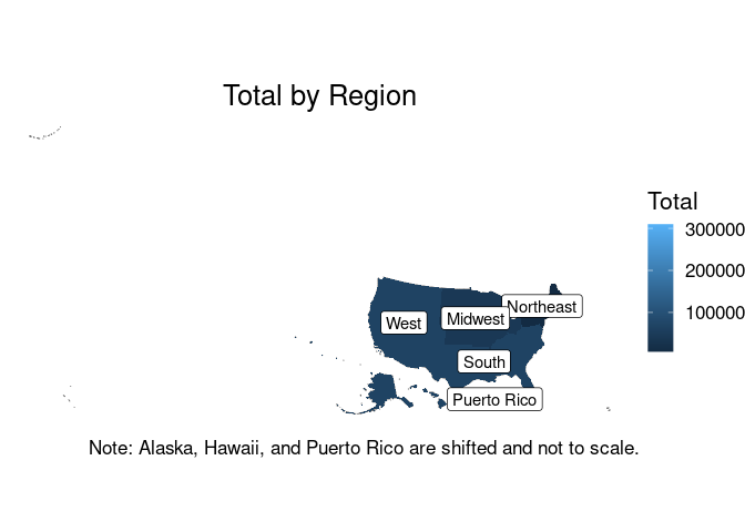
region_data %>% kable()
| REGION | geometry | total |
|---|---|---|
| Northeast | MULTIPOLYGON (((2002871 227… | 7065 |
| Midwest | POLYGON ((1057577 2178191, … | 40175 |
| South | MULTIPOLYGON (((1331106 268… | 66847 |
| West | MULTIPOLYGON (((-2614144 -8… | 66722 |
| Puerto Rico | MULTIPOLYGON (((3369551 -16… | NA |
| Other | GEOMETRYCOLLECTION EMPTY | 309551 |
Created on 2021-09-19 by the reprex package (v2.0.1)
