why is pbinom giving 2 different results for the same proportion?

[brennan2018]

I was trying to calculate a cumulative probability with pbinom and got a bunch of weird results.
why is pbinom giving 2 different results for the same proportion?
I believe pbinom do it correctly. but I don't know what formula pbinom is using.
could any one give a formula to do it correctly?

pbinom(35,100,.3)
[1] 0.8839214
pbinom(350,1000,.3)
[1] 0.9997076

pbinom(35,100,.5)
[1] 0.001758821
pbinom(350,1000,.5)
[1] 8.078155e-22

[joels]

The probability distribution for 350 successes out of 1,000 trials is much more sharply peaked than the distribution of 35 successes out of 100 trials, even though they both represent a 35% success rate.

The formula for the cumulative distribution function is:

You can calculate this directly in R using the code below. The choose() function is the \binom{n}{k} in the formula above. It represents the number of ways to choose k out of n elements.

sum(choose(100, 0:35) * 0.5^(0:35) * 0.5^(100:65))
#> [1] 0.001758821
sum(choose(1000, 0:350) * 0.5^(0:350) * 0.5^(1000:650))
#> [1] 8.078155e-22

^{Created on 2018-12-06 by the reprex package (v0.2.1)}

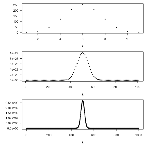
In the examples below, note how the number of ways to choose k out of n elements becomes more peaked as n increases. The vertical axis is \binom{n}{k} for each k:

par(mfrow=c(3,1))
plot(choose(10, 0:10), pch=16, cex=0.7, las=1, ylab="", xlab="k")
plot(choose(100, 0:100), pch=16, cex=0.7, las=1, ylab="", xlab="k")
plot(choose(1000,0:1000), pch=16, cex=0.7, las=1, ylab="", xlab="k")

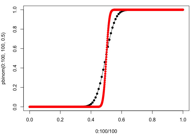
And here's a graphical example of the cumulative distribution function from your example:

plot(0:100/100, pbinom(0:100, 100, 0.5), type="o", pch=16)

lines(0:1000/1000, pbinom(0:1000, 1000, 0.5), col="red")
points(0:1000/1000, pbinom(0:1000, 1000, 0.5), col="red", pch=16)

[technocrat]

(post withdrawn by author, will be automatically deleted in 24 hours unless flagged)