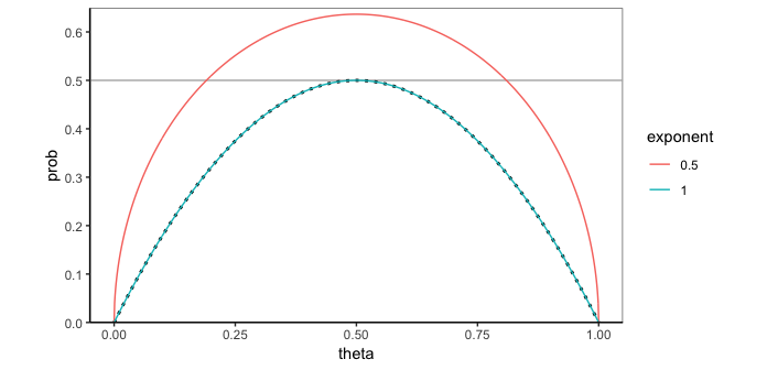
Interesting. I don't have an intuitive explanation and don't know whether the relationship to a circle is coincidental. Your example can be thought of as the probability of 0.5 successes in 1 trial (save for the missing binomial coefficient), which isn't meaningful for a discrete probability. However, if we proceed formally using the generalized binomial expansion, we can calculate what the "probability density" would be in an abstract, formal way.
Below is a function that calculates the generalized binomial probability for an equal number of successes and failures at a range of theta values (where theta is the probability of success in each trial). The function argument n is the number trials, which is 1 in your example, but would be an even number if we wanted only "real" probabilities.
# Return the probability of an equal number of successes and failures for any
# number of "trials", where the argument n is the number of trials. n can be
# any real number (it can even be a complex number in general, but the
# function isn't set up to work with complex numbers)
generalized.dbinom = function(n) {

  # The parameter for the success probability in the binomial distribution
  theta = seq(0,1,0.001)

  # The generalized binomial coefficient (see link above)
  binom.coef = gamma(n + 1)/(gamma(n/2 + 1)*gamma(n - n/2 + 1))

  # The product of the probability of success in all the trials
  prob = (theta*(1 - theta))^(n/2)

  # Return a data frame with the results
  data.frame(theta, prob=prob*binom.coef)
}
The code below plots the output of the function for your example, and for the real-world case of 1 success in 2 trials. The extra call to geom_line using dbinom is there just to show that the generalized binomial function gives the same result as dbinom in a standard discrete-probability case.
library(tidyverse)
theme_set(theme_classic())

ggplot(map_df(c(1,2) %>% set_names(./2), generalized.dbinom, .id="exponent"),
       aes(theta, prob)) +
  geom_hline(yintercept = 0.5, colour="grey70") +
  geom_line(data=tibble(theta=seq(0,1,0.01), prob=dbinom(1,2,theta)),
            linetype="12", size=1) +
  geom_line(aes(colour=exponent)) +
  scale_y_continuous(expand=expand_scale(mult=c(0,0.02)), breaks=seq(0,1,0.1)) +
  coord_equal()