Which models to use when forecasting autocorrelated time series data that shows exponential decay?

I am working through Hyndman, R.J., & Athanasopoulos, G. (2021) Forecasting: principles and practice , 3rd edition, OTexts: Melbourne, Australia. Forecasting: Principles and Practice (3rd ed) (accessed on 30 January 2023). I am interested in generating point and interval forecasts for autocorrelated, non-seasonal time series data that shows exponential decay when expressed as unit transitions to "State X", and otherwise a logarithmic function when those unit transitions are instead expressed as a percentage of initial population units (basically reversing the exponential decay curve). As a frequent user of Stack Overflow I posted a related question on r - Which models to use when forecasting time series data that shows exponential decay? - Cross Validated.

I've been going through the list of models available in the fable package (Forecasting Models for Tidy Time Series • fable) and am having trouble figuring out if there is a better type of model suited for my exponential decay situation (or its logarithmic corollary when expressed as a percentage of initial units in the population). Is there a type of model better suited for this type of data? I've been working through ARIMA, RW, and ETS models so far.


Referred here by Forecasting: Principles and Practice, by Rob J Hyndman and George Athanasopoulos
Using one of the autocorrelation tests on model results to see if there is a need to do first- or second-order differencing or seasonal differencing?

Do you have series data that correlates with the variable being analyzed, such as air conditioning demand in cooling days over the course of the transition from summer to winter? If so, a TSLM might be appropriate.

Regardless of the models I expect to explore, I always do a reference set of naive, seasonal naive, mean, random walk to set a benchmark.

A decay in signal ought to reflect a trend after accounting for seasonality and setting aside residuals. That leads to looking at smoothing methods. If the trend is an exponential decay plus noise how to proceed depends on how close to an asymptote the trend appears. Alternatively, ARIMA looks at integration, rather than differencing and for the non-seasonal case, there are the five special cases of ARIMA shown in Table 9.1 of the book.

Hi Technocrat. Thank you for the feedback. The autocorrelation tests I've run show a need for first-order differencing. With regards to the point in your 2nd paragraph, there is no series data that correlates with the variable being analyzed. With regards to your 3rd paragraph, I'm working through naive, naive with drift, mean, and random walk models; I'm getting best results with naive with drift and RW. There is no seasonality in the data, only trend + noise. The trend is exponential decay with noise -- the data usually approaches 0 gradually over time without ever reaching 0 (asymptote). In your 4th paragraph you say "how to proceed depends on how close to an asymptote the trend appears...": what do you see as the model options to follow for proceeding, assuming the trend is close to an asymptote?

So, maybe a Box-Cox to make stationary, can't use a TSLM model to add a condition like, say, temperature in an energy forecasting model.

The four baselines are what I use.

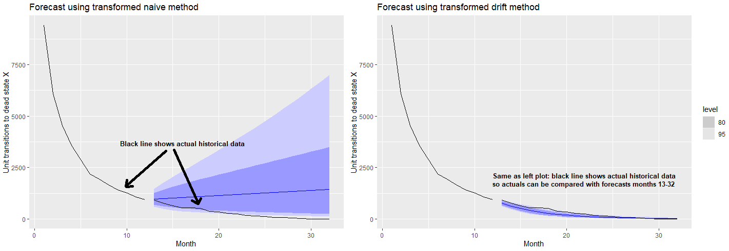
As the trend line declines, at some point with a given forecast horizon, the confidence bands will reach zero before the decay curve. That becomes a problem of assessing confidence in the data, perhaps some explanatory rationale for the historical shape of the data and the relative dangers of picking a cutoff ignoring the confidence bands or setting it at some x-intercept that is "close enough" without running into the confidence band limitations. How do your CIs plot out?

The data is "survival data"; elements transition to dead-state X over 32 months, with the most unit transitions in the early months following an exponential decay curve through the 32 months. By month 32 transitions in the historical dataset used in this analysis reach 0; but in the larger population as a whole this is not always necessarily so. I'm forecasting "as-if" I had only the first 12 months of data, and then I compare those forecasts with actual data for "assumed future" months 13-32. Ultimately my goal is to run simulations where I draw a histogram of a probability distribution of cumulative transitions during those forecast months 13-32. Practically speaking, there is more "risk" in my under-forecasting transitions than in over-forecasting, which draws me towards the naive method instead of drift although naive does seem quite severe. Below I show CI for log-transformed naive and drift methods, and I also show residual diagnostic graphs for both. I use log transformations because negative transitions are impossible; there is no coming back from the dead state. At the very bottom I also post the data and R code used to generate these graphics.


R code:

library(dplyr)
library(fabletools)
library(fable)
library(feasts)
library(ggplot2)
library(ggnewscale)
library(tidyr)
library(tsibble)

data <- data.frame(
  Month =c(1:32),
  StateX=c(
    9416,6086,4559,3586,2887,2175,1945,1675,1418,1259,1079,940,923,776,638,545,547,510,379,
    341,262,241,168,155,133,76,69,45,17,9,5,0
  ),
  rateCumX=c(
    0.1623159,0.23137659,0.29942238,0.35294557,0.39603576,0.42849893,0.45752922,0.48252959,
    0.50369408,0.52248541,0.53859013,0.55262019,0.56639651,0.57797878,0.58750131,0.59563576,
    0.60380006,0.61141211,0.61706891,0.62215854,0.62606905,0.62966611,0.63217361,0.63448708,
    0.63647219,0.63760653,0.63863640,0.63930805,0.63956178,0.63969611,0.63977074,0.63977074
  )
) %>% 
  as_tsibble(index = Month)

# naive method CI
data[1:12,] %>%
  model(NAIVE(log(StateX))) %>%
  forecast(h = 20) %>%
  autoplot(data[1:12,]) +
  autolayer(
    filter_index(data, 13 ~ .), 
    colour = "black") +
  labs(title="Forecast using transformed naive method", 
       y="Unit transitions to dead state X")

# drift method CI
data[1:12,] %>%
  model(NAIVE(log(StateX)~drift())) %>%
  forecast(h = 20) %>%
  autoplot(data[1:12,]) +
  autolayer(
    filter_index(data, 13 ~ .), 
    colour = "black") +
  labs(title="Forecast using transformed drift method", 
       y="Unit transitions to dead state X")

# residual diagnostics for naive method
data[1:12,] %>%
  model(NAIVE(log(StateX))) %>%
  gg_tsresiduals()

# residual diagnostics for drift method
data[1:12,] %>%
  model(NAIVE(log(StateX)~drift())) %>%
  gg_tsresiduals()

This topic was automatically closed 21 days after the last reply. New replies are no longer allowed.

If you have a query related to it or one of the replies, start a new topic and refer back with a link.