What is the main difference between lm() and VIF (between 1 factor and 1 cont. variable)?

[Nate_L]

I know this isn't a coding question, so I apologize if it's too off topic. I'm confused because I don't understand why an ANOVA/linear model would give a different answer than VIF of a simple linear model with 2 predictor variables. For example, if I want to know if water temp. (a continuous covariate) is too closely related to a factor variable "season" to be put into the same model to predict some other variable (3rd variable not important here), what's the best way to tell? Obviously water temp. and season would seem too related, but choose any 2 variables! How does one test one continuous variable and a factor for similarities when it's not obvious? What is the best way to answer "are these two too closely related to be in the same model?"(?) Why isn't the VIF "test" telling me these are too related (VIF is less than 4!), like the linear model (at least in a different way)?

library(gratia)
library(performance)

df <- as.data.frame(rnorm(50, mean = 23.8, sd = 2.60))
df2 <- as.data.frame(rnorm(50, mean = 30.2, sd = 1.62))

names(df)[1] <- "temp"
names(df2)[1] <- "temp"
df3 <- rbind(df, df2)

df3$season <- rep(c("DRY", "WET"), each=50)

x <- rnorm(100, mean=0, sd=1)
df3$x <- x

full <- lm(x ~ temp + season, data=df3)

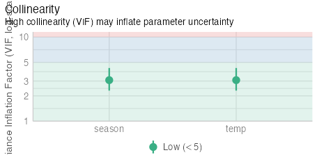
vif.cat.data <- check_collinearity(full)
vif.cat.data
# Check for Multicollinearity

Low Correlation

   Term  VIF   VIF 95% CI Increased SE Tolerance Tolerance 95% CI
   temp 3.04 [2.28, 4.23]         1.74      0.33     [0.24, 0.44]
 season 3.04 [2.28, 4.23]         1.74      0.33     [0.24, 0.44]
# NOT too closely related!?

###############################################################################

# Now with ANOVA/linear model
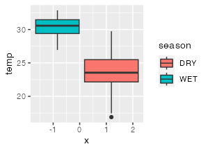
lm <- lm(temp ~ season, data=df3)
summary(lm)

Call:
lm(formula = temp ~ season, data = df3)

Residuals:
    Min      1Q  Median      3Q     Max 
-5.9874 -0.9893 -0.0597  1.1201  5.1884 

Coefficients:
            Estimate Std. Error t value Pr(>|t|)    
(Intercept)  24.8731     0.2729   91.14   <2e-16 ***
seasonWET     5.4516     0.3860   14.12   <2e-16 ***
---
Signif. codes:  0 ‘***’ 0.001 ‘**’ 0.01 ‘*’ 0.05 ‘.’ 0.1 ‘ ’ 1

Residual standard error: 1.93 on 98 degrees of freedom
Multiple R-squared:  0.6706,	Adjusted R-squared:  0.6672 # <--Definitely related?? 
F-statistic: 199.5 on 1 and 98 DF,  p-value: < 2.2e-16

[Nate_L]

Is this equation correct? It certainly seems to answer my question

#VIF function
r<-function(x){1-(1/x)} #r is R2 and x is VIF
x<-seq(1,15,.1) #seq of VIFs
y<-sapply(x,r) #seq of R2
#plot
par(las=1)
plot(x,y,type="l",xlab="VIF",ylab="R2 of regression of focal covariate on all other covariates")
# common VIF cutoffs = 2.5, 5, 10
ly<-c(y[x==2.5],y[x==5],y[x==10])
lx<-c(2.5,5,10)
segments(lx,0,lx,ly,col="red")
segments(lx,ly,0,ly,col="red")

Source: https://haotu.wordpress.com/2016/10/28/the-relationship-between-vif-and-r2-r-squared/

[technocrat]

As far as I'm concerned, R and statistics are BFFs and there can be no reason to separate the coding aspects of using it from the domain aspects. Because, frankly, there are better general purpose coding languages than R out there. Open-source languages for applied statistics? Not too much competition

ANOVA answers the question: given two vectors, are their means difference for some selection of \alpha (aka, the unfortunately named significance.

VIF answers the question: in an ordinary least squares regression model involving multiple independent variables, to what extent do the variables increase the variance of parameters. In other words, is there double dipping? That's the gist of the collinearity issue.

So, are the two telling us anything different?

library(ggplot2)
#> Warning: package 'ggplot2' was built under R version 4.3.1
library(gratia)
library(multcompView)
library(performance)
library(see)

set.seed(42)
df_ <- as.data.frame(rnorm(50, mean = 23.8, sd = 2.60))
set.seed(137)
df2 <- as.data.frame(rnorm(50, mean = 30.2, sd = 1.62))

names(df_)[1] <- "temp"
names(df2)[1] <- "temp"
df3 <- rbind(df_, df2)

df3$season <- rep(c("DRY", "WET"), each=50)

set.seed(173)
x <- rnorm(100, mean=0, sd=1)
df3$x <- x

full <- lm(x ~ temp + season, data=df3)
(vif.cat.data <- check_collinearity(full))
#> # Check for Multicollinearity
#> 
#> Low Correlation
#> 
#>    Term  VIF   VIF 95% CI Increased SE Tolerance Tolerance 95% CI
#>    temp 3.07 [2.31, 4.29]         1.75      0.33     [0.23, 0.43]
#>  season 3.07 [2.31, 4.29]         1.75      0.33     [0.23, 0.43]
plot(vif.cat.data)
#> Variable `Component` is not in your data frame :/

result <- aov(temp ~ season, data=df3)
summary(result)
#>             Df Sum Sq Mean Sq F value Pr(>F)    
#> season       1   1112  1112.0   203.3 <2e-16 ***
#> Residuals   98    536     5.5                   
#> ---
#> Signif. codes:  0 '***' 0.001 '**' 0.01 '*' 0.05 '.' 0.1 ' ' 1
ggplot(df3, aes(x = x, y = temp)) +
  geom_boxplot(aes(fill = season))

^{Created on 2023-10-21 with reprex v2.0.2}

So, I've substituted aov for lm, because we want to get apples and apples. But, given that the variables are, by design, random, the results show what we expect. The means of the two independent variables differ, as we'd expect—random continuous variable vs. random binary variable, and their collinearity is low. So, I'd say that the two statistical tests point in the same direction: there is no reason to exclude a variable.

Of course, the data are random. Real data may differ.

[Nate_L]

Great points, thank you!!