Hi,
I estimated in total 10 ordered logit regressiona using the polr function and I have 10 variables in each where most of them have many categories. So, I do not think it make sense to determine each proability. However, the intercepts itself are not so much useable (as far I understooth).
Do you have any suggestions/recommendation for what I can do? What are the options using R?
The polr is from the MASS package, just to let you know.
Run the examples from help(polr), shown below in the reprex. To better understand them, read through the rest of the help page carefully. If still uncertain read one or both of
Agresti, A. (2002) Categorical Data. Second edition. Wiley.
Venables, W. N. and Ripley, B. D. (2002) Modern Applied Statistics with S. Fourth edition. Springer.
or a text with similar coverage. If those are not helpful, it is probably necessary to get some formal instruction. We should never use features of R that we don't fully understand.
library(MASS)
options(contrasts = c("contr.treatment", "contr.poly"))
house.plr <- polr(Sat ~ Infl + Type + Cont, weights = Freq, data = housing)
house.plr
#> Call:
#> polr(formula = Sat ~ Infl + Type + Cont, data = housing, weights = Freq)
#>
#> Coefficients:
#> InflMedium InflHigh TypeApartment TypeAtrium TypeTerrace
#> 0.5663937 1.2888191 -0.5723501 -0.3661866 -1.0910149
#> ContHigh
#> 0.3602841
#>
#> Intercepts:
#> Low|Medium Medium|High
#> -0.4961353 0.6907083
#>
#> Residual Deviance: 3479.149
#> AIC: 3495.149
summary(house.plr, digits = 3)
#>
#> Re-fitting to get Hessian
#> Call:
#> polr(formula = Sat ~ Infl + Type + Cont, data = housing, weights = Freq)
#>
#> Coefficients:
#> Value Std. Error t value
#> InflMedium 0.566 0.1047 5.41
#> InflHigh 1.289 0.1272 10.14
#> TypeApartment -0.572 0.1192 -4.80
#> TypeAtrium -0.366 0.1552 -2.36
#> TypeTerrace -1.091 0.1515 -7.20
#> ContHigh 0.360 0.0955 3.77
#>
#> Intercepts:
#> Value Std. Error t value
#> Low|Medium -0.496 0.125 -3.974
#> Medium|High 0.691 0.125 5.505
#>
#> Residual Deviance: 3479.149
#> AIC: 3495.149
## slightly worse fit from
summary(update(house.plr, method = "probit", Hess = TRUE), digits = 3)
#> Call:
#> polr(formula = Sat ~ Infl + Type + Cont, data = housing, weights = Freq,
#> Hess = TRUE, method = "probit")
#>
#> Coefficients:
#> Value Std. Error t value
#> InflMedium 0.346 0.0641 5.40
#> InflHigh 0.783 0.0764 10.24
#> TypeApartment -0.348 0.0723 -4.81
#> TypeAtrium -0.218 0.0948 -2.30
#> TypeTerrace -0.664 0.0918 -7.24
#> ContHigh 0.222 0.0581 3.83
#>
#> Intercepts:
#> Value Std. Error t value
#> Low|Medium -0.300 0.076 -3.937
#> Medium|High 0.427 0.076 5.585
#>
#> Residual Deviance: 3479.689
#> AIC: 3495.689
## although it is not really appropriate, can fit
summary(update(house.plr, method = "loglog", Hess = TRUE), digits = 3)
#> Call:
#> polr(formula = Sat ~ Infl + Type + Cont, data = housing, weights = Freq,
#> Hess = TRUE, method = "loglog")
#>
#> Coefficients:
#> Value Std. Error t value
#> InflMedium 0.367 0.0727 5.05
#> InflHigh 0.790 0.0806 9.81
#> TypeApartment -0.349 0.0757 -4.61
#> TypeAtrium -0.196 0.0988 -1.98
#> TypeTerrace -0.698 0.1043 -6.69
#> ContHigh 0.268 0.0636 4.21
#>
#> Intercepts:
#> Value Std. Error t value
#> Low|Medium 0.086 0.083 1.038
#> Medium|High 0.892 0.087 10.223
#>
#> Residual Deviance: 3491.41
#> AIC: 3507.41
summary(update(house.plr, method = "cloglog", Hess = TRUE), digits = 3)
#> Call:
#> polr(formula = Sat ~ Infl + Type + Cont, data = housing, weights = Freq,
#> Hess = TRUE, method = "cloglog")
#>
#> Coefficients:
#> Value Std. Error t value
#> InflMedium 0.382 0.0703 5.44
#> InflHigh 0.915 0.0926 9.89
#> TypeApartment -0.407 0.0861 -4.73
#> TypeAtrium -0.281 0.1111 -2.52
#> TypeTerrace -0.742 0.1013 -7.33
#> ContHigh 0.209 0.0651 3.21
#>
#> Intercepts:
#> Value Std. Error t value
#> Low|Medium -0.796 0.090 -8.881
#> Medium|High 0.055 0.086 0.647
#>
#> Residual Deviance: 3484.053
#> AIC: 3500.053
predict(house.plr, housing, type = "p")
#> Low Medium High
#> 1 0.3784493 0.2876752 0.3338755
#> 2 0.3784493 0.2876752 0.3338755
#> 3 0.3784493 0.2876752 0.3338755
#> 4 0.2568264 0.2742122 0.4689613
#> 5 0.2568264 0.2742122 0.4689613
#> 6 0.2568264 0.2742122 0.4689613
#> 7 0.1436924 0.2110836 0.6452240
#> 8 0.1436924 0.2110836 0.6452240
#> 9 0.1436924 0.2110836 0.6452240
#> 10 0.5190445 0.2605077 0.2204478
#> 11 0.5190445 0.2605077 0.2204478
#> 12 0.5190445 0.2605077 0.2204478
#> 13 0.3798514 0.2875965 0.3325521
#> 14 0.3798514 0.2875965 0.3325521
#> 15 0.3798514 0.2875965 0.3325521
#> 16 0.2292406 0.2643196 0.5064398
#> 17 0.2292406 0.2643196 0.5064398
#> 18 0.2292406 0.2643196 0.5064398
#> 19 0.4675584 0.2745383 0.2579033
#> 20 0.4675584 0.2745383 0.2579033
#> 21 0.4675584 0.2745383 0.2579033
#> 22 0.3326236 0.2876008 0.3797755
#> 23 0.3326236 0.2876008 0.3797755
#> 24 0.3326236 0.2876008 0.3797755
#> 25 0.1948548 0.2474226 0.5577225
#> 26 0.1948548 0.2474226 0.5577225
#> 27 0.1948548 0.2474226 0.5577225
#> 28 0.6444840 0.2114256 0.1440905
#> 29 0.6444840 0.2114256 0.1440905
#> 30 0.6444840 0.2114256 0.1440905
#> 31 0.5071210 0.2641196 0.2287594
#> 32 0.5071210 0.2641196 0.2287594
#> 33 0.5071210 0.2641196 0.2287594
#> 34 0.3331573 0.2876330 0.3792097
#> 35 0.3331573 0.2876330 0.3792097
#> 36 0.3331573 0.2876330 0.3792097
#> 37 0.2980880 0.2837746 0.4181374
#> 38 0.2980880 0.2837746 0.4181374
#> 39 0.2980880 0.2837746 0.4181374
#> 40 0.1942209 0.2470589 0.5587202
#> 41 0.1942209 0.2470589 0.5587202
#> 42 0.1942209 0.2470589 0.5587202
#> 43 0.1047770 0.1724227 0.7228003
#> 44 0.1047770 0.1724227 0.7228003
#> 45 0.1047770 0.1724227 0.7228003
#> 46 0.4294564 0.2820629 0.2884807
#> 47 0.4294564 0.2820629 0.2884807
#> 48 0.4294564 0.2820629 0.2884807
#> 49 0.2993357 0.2839753 0.4166890
#> 50 0.2993357 0.2839753 0.4166890
#> 51 0.2993357 0.2839753 0.4166890
#> 52 0.1718050 0.2328648 0.5953302
#> 53 0.1718050 0.2328648 0.5953302
#> 54 0.1718050 0.2328648 0.5953302
#> 55 0.3798387 0.2875972 0.3325641
#> 56 0.3798387 0.2875972 0.3325641
#> 57 0.3798387 0.2875972 0.3325641
#> 58 0.2579546 0.2745537 0.4674917
#> 59 0.2579546 0.2745537 0.4674917
#> 60 0.2579546 0.2745537 0.4674917
#> 61 0.1444202 0.2117081 0.6438717
#> 62 0.1444202 0.2117081 0.6438717
#> 63 0.1444202 0.2117081 0.6438717
#> 64 0.5583813 0.2471826 0.1944361
#> 65 0.5583813 0.2471826 0.1944361
#> 66 0.5583813 0.2471826 0.1944361
#> 67 0.4178031 0.2838213 0.2983756
#> 68 0.4178031 0.2838213 0.2983756
#> 69 0.4178031 0.2838213 0.2983756
#> 70 0.2584149 0.2746916 0.4668935
#> 71 0.2584149 0.2746916 0.4668935
#> 72 0.2584149 0.2746916 0.4668935
addterm(house.plr, ~.^2, test = "Chisq")
#> Single term additions
#>
#> Model:
#> Sat ~ Infl + Type + Cont
#> Df AIC LRT Pr(Chi)
#> <none> 3495.1
#> Infl:Type 6 3484.6 22.5093 0.0009786 ***
#> Infl:Cont 2 3498.9 0.2090 0.9007957
#> Type:Cont 3 3492.5 8.6662 0.0340752 *
#> ---
#> Signif. codes: 0 '***' 0.001 '**' 0.01 '*' 0.05 '.' 0.1 ' ' 1
house.plr2 <- stepAIC(house.plr, ~.^2)
#> Start: AIC=3495.15
#> Sat ~ Infl + Type + Cont
#>
#> Df AIC
#> + Infl:Type 6 3484.6
#> + Type:Cont 3 3492.5
#> <none> 3495.1
#> + Infl:Cont 2 3498.9
#> - Cont 1 3507.5
#> - Type 3 3545.1
#> - Infl 2 3599.4
#>
#> Step: AIC=3484.64
#> Sat ~ Infl + Type + Cont + Infl:Type
#>
#> Df AIC
#> + Type:Cont 3 3482.7
#> <none> 3484.6
#> + Infl:Cont 2 3488.5
#> - Infl:Type 6 3495.1
#> - Cont 1 3497.8
#>
#> Step: AIC=3482.69
#> Sat ~ Infl + Type + Cont + Infl:Type + Type:Cont
#>
#> Df AIC
#> <none> 3482.7
#> - Type:Cont 3 3484.6
#> + Infl:Cont 2 3486.6
#> - Infl:Type 6 3492.5
house.plr2$anova
#> Stepwise Model Path
#> Analysis of Deviance Table
#>
#> Initial Model:
#> Sat ~ Infl + Type + Cont
#>
#> Final Model:
#> Sat ~ Infl + Type + Cont + Infl:Type + Type:Cont
#>
#>
#> Step Df Deviance Resid. Df Resid. Dev AIC
#> 1 1673 3479.149 3495.149
#> 2 + Infl:Type 6 22.509347 1667 3456.640 3484.640
#> 3 + Type:Cont 3 7.945029 1664 3448.695 3482.695
anova(house.plr, house.plr2)
#> Likelihood ratio tests of ordinal regression models
#>
#> Response: Sat
#> Model Resid. df Resid. Dev Test Df
#> 1 Infl + Type + Cont 1673 3479.149
#> 2 Infl + Type + Cont + Infl:Type + Type:Cont 1664 3448.695 1 vs 2 9
#> LR stat. Pr(Chi)
#> 1
#> 2 30.45438 0.0003670555
house.plr <- update(house.plr, Hess=TRUE)
pr <- profile(house.plr)
confint(pr)
#> 2.5 % 97.5 %
#> InflMedium 0.3616415 0.77195375
#> InflHigh 1.0409701 1.53958138
#> TypeApartment -0.8069590 -0.33940432
#> TypeAtrium -0.6705862 -0.06204495
#> TypeTerrace -1.3893863 -0.79533958
#> ContHigh 0.1733589 0.54792854
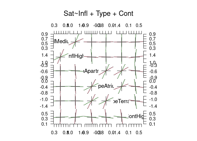
plot(pr)

pairs(pr)
Created on 2022-11-17 by the reprex package (v2.0.1)
Thanks, I will have a look at these books. Can you explain what these two plots shows/indicate?
Sorry, that I was to early for asking before I do my own reaserch.. as far I understooth the second plot is actually a scatterplot.. then it can be used to detect outliers, right? However the second plot I still do not know how to interpret.. the same for the first plot.
That's right, an x-vector against a y-vector, derived from the pr object, which is of profile.polr, which is a very complex object. I can't tell just from looking at it which two vectors are being plotted and wouldn't use it until I understood.
library(MASS)
options(contrasts = c("contr.treatment", "contr.poly"))
house.plr <- polr(Sat ~ Infl + Type + Cont, weights = Freq, data = housing)
house.plr <- update(house.plr, Hess=TRUE)
pr <- profile(house.plr)
str(pr)
#> List of 6
#>  $ InflMedium   :'data.frame':   12 obs. of  2 variables:
#>   ..$ z       : num [1:12] -2.582 -2.064 -1.548 -1.031 -0.515 ...
#>   ..$ par.vals: num [1:12, 1:6] 0.297 0.351 0.405 0.459 0.512 ...
#>   .. ..- attr(*, "dimnames")=List of 2
#>   .. .. ..$ : NULL
#>   .. .. ..$ : chr [1:6] "InflMedium" "InflHigh" "TypeApartment" "TypeAtrium" ...
#>  $ InflHigh     :'data.frame':   12 obs. of  2 variables:
#>   ..$ z       : num [1:12] -2.594 -2.073 -1.552 -1.033 -0.516 ...
#>   ..$ par.vals: num [1:12, 1:6] 0.447 0.471 0.495 0.519 0.543 ...
#>   .. ..- attr(*, "dimnames")=List of 2
#>   .. .. ..$ : NULL
#>   .. .. ..$ : chr [1:6] "InflMedium" "InflHigh" "TypeApartment" "TypeAtrium" ...
#>  $ TypeApartment:'data.frame':   12 obs. of  2 variables:
#>   ..$ z       : num [1:12] -3.07 -2.56 -2.05 -1.54 -1.03 ...
#>   ..$ par.vals: num [1:12, 1:6] 0.572 0.57 0.569 0.568 0.568 ...
#>   .. ..- attr(*, "dimnames")=List of 2
#>   .. .. ..$ : NULL
#>   .. .. ..$ : chr [1:6] "InflMedium" "InflHigh" "TypeApartment" "TypeAtrium" ...
#>  $ TypeAtrium   :'data.frame':   13 obs. of  2 variables:
#>   ..$ z       : num [1:13] -3.09 -2.57 -2.06 -1.54 -1.03 ...
#>   ..$ par.vals: num [1:13, 1:6] 0.562 0.562 0.563 0.563 0.564 ...
#>   .. ..- attr(*, "dimnames")=List of 2
#>   .. .. ..$ : NULL
#>   .. .. ..$ : chr [1:6] "InflMedium" "InflHigh" "TypeApartment" "TypeAtrium" ...
#>  $ TypeTerrace  :'data.frame':   12 obs. of  2 variables:
#>   ..$ z       : num [1:12] -3.07 -2.56 -2.05 -1.54 -1.03 ...
#>   ..$ par.vals: num [1:12, 1:6] 0.566 0.566 0.566 0.566 0.566 ...
#>   .. ..- attr(*, "dimnames")=List of 2
#>   .. .. ..$ : NULL
#>   .. .. ..$ : chr [1:6] "InflMedium" "InflHigh" "TypeApartment" "TypeAtrium" ...
#>  $ ContHigh     :'data.frame':   12 obs. of  2 variables:
#>   ..$ z       : num [1:12] -2.581 -2.064 -1.548 -1.031 -0.515 ...
#>   ..$ par.vals: num [1:12, 1:6] 0.554 0.556 0.558 0.561 0.564 ...
#>   .. ..- attr(*, "dimnames")=List of 2
#>   .. .. ..$ : NULL
#>   .. .. ..$ : chr [1:6] "InflMedium" "InflHigh" "TypeApartment" "TypeAtrium" ...
#>  - attr(*, "original.fit")=List of 19
#>   ..$ coefficients : Named num [1:6] 0.566 1.289 -0.572 -0.366 -1.091 ...
#>   .. ..- attr(*, "names")= chr [1:6] "InflMedium" "InflHigh" "TypeApartment" "TypeAtrium" ...
#>   ..$ zeta         : Named num [1:2] -0.496 0.691
#>   .. ..- attr(*, "names")= chr [1:2] "Low|Medium" "Medium|High"
#>   ..$ deviance     : num 3479
#>   ..$ fitted.values: num [1:72, 1:3] 0.378 0.378 0.378 0.257 0.257 ...
#>   .. ..- attr(*, "dimnames")=List of 2
#>   .. .. ..$ : chr [1:72] "1" "2" "3" "4" ...
#>   .. .. ..$ : chr [1:3] "Low" "Medium" "High"
#>   ..$ lev          : chr [1:3] "Low" "Medium" "High"
#>   ..$ terms        :Classes 'terms', 'formula'  language Sat ~ Infl + Type + Cont
#>   .. .. ..- attr(*, "variables")= language list(Sat, Infl, Type, Cont)
#>   .. .. ..- attr(*, "factors")= int [1:4, 1:3] 0 1 0 0 0 0 1 0 0 0 ...
#>   .. .. .. ..- attr(*, "dimnames")=List of 2
#>   .. .. .. .. ..$ : chr [1:4] "Sat" "Infl" "Type" "Cont"
#>   .. .. .. .. ..$ : chr [1:3] "Infl" "Type" "Cont"
#>   .. .. ..- attr(*, "term.labels")= chr [1:3] "Infl" "Type" "Cont"
#>   .. .. ..- attr(*, "order")= int [1:3] 1 1 1
#>   .. .. ..- attr(*, "intercept")= int 1
#>   .. .. ..- attr(*, "response")= int 1
#>   .. .. ..- attr(*, ".Environment")=<environment: R_GlobalEnv>
#>   .. .. ..- attr(*, "predvars")= language list(Sat, Infl, Type, Cont)
#>   .. .. ..- attr(*, "dataClasses")= Named chr [1:5] "ordered" "factor" "factor" "factor" ...
#>   .. .. .. ..- attr(*, "names")= chr [1:5] "Sat" "Infl" "Type" "Cont" ...
#>   ..$ df.residual  : int 1673
#>   ..$ edf          : int 8
#>   ..$ n            : int 1681
#>   ..$ nobs         : int 1681
#>   ..$ call         : language polr(formula = Sat ~ Infl + Type + Cont, data = housing, weights = Freq,      Hess = TRUE)
#>   ..$ method       : chr "logistic"
#>   ..$ convergence  : int 0
#>   ..$ niter        : Named int [1:2] 51 13
#>   .. ..- attr(*, "names")= chr [1:2] "f.evals.function" "g.evals.gradient"
#>   ..$ lp           : Named num [1:72] 0 0 0 0.566 0.566 ...
#>   .. ..- attr(*, "names")= chr [1:72] "1" "2" "3" "4" ...
#>   ..$ Hessian      : num [1:8, 1:8] 190.5 0 86.4 25.8 31.4 ...
#>   .. ..- attr(*, "dimnames")=List of 2
#>   .. .. ..$ : chr [1:8] "InflMedium" "InflHigh" "TypeApartment" "TypeAtrium" ...
#>   .. .. ..$ : chr [1:8] "InflMedium" "InflHigh" "TypeApartment" "TypeAtrium" ...
#>   ..$ model        :'data.frame':    72 obs. of  5 variables:
#>   .. ..$ Sat      : Ord.factor w/ 3 levels "Low"<"Medium"<..: 1 2 3 1 2 3 1 2 3 1 ...
#>   .. ..$ Infl     : Factor w/ 3 levels "Low","Medium",..: 1 1 1 2 2 2 3 3 3 1 ...
#>   .. ..$ Type     : Factor w/ 4 levels "Tower","Apartment",..: 1 1 1 1 1 1 1 1 1 2 ...
#>   .. ..$ Cont     : Factor w/ 2 levels "Low","High": 1 1 1 1 1 1 1 1 1 1 ...
#>   .. ..$ (weights): int [1:72] 21 21 28 34 22 36 10 11 36 61 ...
#>   .. ..- attr(*, "terms")=Classes 'terms', 'formula'  language Sat ~ Infl + Type + Cont
#>   .. .. .. ..- attr(*, "variables")= language list(Sat, Infl, Type, Cont)
#>   .. .. .. ..- attr(*, "factors")= int [1:4, 1:3] 0 1 0 0 0 0 1 0 0 0 ...
#>   .. .. .. .. ..- attr(*, "dimnames")=List of 2
#>   .. .. .. .. .. ..$ : chr [1:4] "Sat" "Infl" "Type" "Cont"
#>   .. .. .. .. .. ..$ : chr [1:3] "Infl" "Type" "Cont"
#>   .. .. .. ..- attr(*, "term.labels")= chr [1:3] "Infl" "Type" "Cont"
#>   .. .. .. ..- attr(*, "order")= int [1:3] 1 1 1
#>   .. .. .. ..- attr(*, "intercept")= int 1
#>   .. .. .. ..- attr(*, "response")= int 1
#>   .. .. .. ..- attr(*, ".Environment")=<environment: R_GlobalEnv>
#>   .. .. .. ..- attr(*, "predvars")= language list(Sat, Infl, Type, Cont)
#>   .. .. .. ..- attr(*, "dataClasses")= Named chr [1:5] "ordered" "factor" "factor" "factor" ...
#>   .. .. .. .. ..- attr(*, "names")= chr [1:5] "Sat" "Infl" "Type" "Cont" ...
#>   ..$ contrasts    :List of 3
#>   .. ..$ Infl: chr "contr.treatment"
#>   .. ..$ Type: chr "contr.treatment"
#>   .. ..$ Cont: chr "contr.treatment"
#>   ..$ xlevels      :List of 3
#>   .. ..$ Infl: chr [1:3] "Low" "Medium" "High"
#>   .. ..$ Type: chr [1:4] "Tower" "Apartment" "Atrium" "Terrace"
#>   .. ..$ Cont: chr [1:2] "Low" "High"
#>   ..- attr(*, "class")= chr "polr"
#>  - attr(*, "summary")=List of 21
#>   ..$ coefficients : num [1:8, 1:3] 0.566 1.289 -0.572 -0.366 -1.091 ...
#>   .. ..- attr(*, "dimnames")=List of 2
#>   .. .. ..$ : chr [1:8] "InflMedium" "InflHigh" "TypeApartment" "TypeAtrium" ...
#>   .. .. ..$ : chr [1:3] "Value" "Std. Error" "t value"
#>   ..$ zeta         : Named num [1:2] -0.496 0.691
#>   .. ..- attr(*, "names")= chr [1:2] "Low|Medium" "Medium|High"
#>   ..$ deviance     : num 3479
#>   ..$ fitted.values: num [1:72, 1:3] 0.378 0.378 0.378 0.257 0.257 ...
#>   .. ..- attr(*, "dimnames")=List of 2
#>   .. .. ..$ : chr [1:72] "1" "2" "3" "4" ...
#>   .. .. ..$ : chr [1:3] "Low" "Medium" "High"
#>   ..$ lev          : chr [1:3] "Low" "Medium" "High"
#>   ..$ terms        :Classes 'terms', 'formula'  language Sat ~ Infl + Type + Cont
#>   .. .. ..- attr(*, "variables")= language list(Sat, Infl, Type, Cont)
#>   .. .. ..- attr(*, "factors")= int [1:4, 1:3] 0 1 0 0 0 0 1 0 0 0 ...
#>   .. .. .. ..- attr(*, "dimnames")=List of 2
#>   .. .. .. .. ..$ : chr [1:4] "Sat" "Infl" "Type" "Cont"
#>   .. .. .. .. ..$ : chr [1:3] "Infl" "Type" "Cont"
#>   .. .. ..- attr(*, "term.labels")= chr [1:3] "Infl" "Type" "Cont"
#>   .. .. ..- attr(*, "order")= int [1:3] 1 1 1
#>   .. .. ..- attr(*, "intercept")= int 1
#>   .. .. ..- attr(*, "response")= int 1
#>   .. .. ..- attr(*, ".Environment")=<environment: R_GlobalEnv>
#>   .. .. ..- attr(*, "predvars")= language list(Sat, Infl, Type, Cont)
#>   .. .. ..- attr(*, "dataClasses")= Named chr [1:5] "ordered" "factor" "factor" "factor" ...
#>   .. .. .. ..- attr(*, "names")= chr [1:5] "Sat" "Infl" "Type" "Cont" ...
#>   ..$ df.residual  : int 1673
#>   ..$ edf          : int 8
#>   ..$ n            : int 1681
#>   ..$ nobs         : int 1681
#>   ..$ call         : language polr(formula = Sat ~ Infl + Type + Cont, data = housing, weights = Freq,      Hess = TRUE)
#>   ..$ method       : chr "logistic"
#>   ..$ convergence  : int 0
#>   ..$ niter        : Named int [1:2] 51 13
#>   .. ..- attr(*, "names")= chr [1:2] "f.evals.function" "g.evals.gradient"
#>   ..$ lp           : Named num [1:72] 0 0 0 0.566 0.566 ...
#>   .. ..- attr(*, "names")= chr [1:72] "1" "2" "3" "4" ...
#>   ..$ Hessian      : num [1:8, 1:8] 190.5 0 86.4 25.8 31.4 ...
#>   .. ..- attr(*, "dimnames")=List of 2
#>   .. .. ..$ : chr [1:8] "InflMedium" "InflHigh" "TypeApartment" "TypeAtrium" ...
#>   .. .. ..$ : chr [1:8] "InflMedium" "InflHigh" "TypeApartment" "TypeAtrium" ...
#>   ..$ model        :'data.frame':    72 obs. of  5 variables:
#>   .. ..$ Sat      : Ord.factor w/ 3 levels "Low"<"Medium"<..: 1 2 3 1 2 3 1 2 3 1 ...
#>   .. ..$ Infl     : Factor w/ 3 levels "Low","Medium",..: 1 1 1 2 2 2 3 3 3 1 ...
#>   .. ..$ Type     : Factor w/ 4 levels "Tower","Apartment",..: 1 1 1 1 1 1 1 1 1 2 ...
#>   .. ..$ Cont     : Factor w/ 2 levels "Low","High": 1 1 1 1 1 1 1 1 1 1 ...
#>   .. ..$ (weights): int [1:72] 21 21 28 34 22 36 10 11 36 61 ...
#>   .. ..- attr(*, "terms")=Classes 'terms', 'formula'  language Sat ~ Infl + Type + Cont
#>   .. .. .. ..- attr(*, "variables")= language list(Sat, Infl, Type, Cont)
#>   .. .. .. ..- attr(*, "factors")= int [1:4, 1:3] 0 1 0 0 0 0 1 0 0 0 ...
#>   .. .. .. .. ..- attr(*, "dimnames")=List of 2
#>   .. .. .. .. .. ..$ : chr [1:4] "Sat" "Infl" "Type" "Cont"
#>   .. .. .. .. .. ..$ : chr [1:3] "Infl" "Type" "Cont"
#>   .. .. .. ..- attr(*, "term.labels")= chr [1:3] "Infl" "Type" "Cont"
#>   .. .. .. ..- attr(*, "order")= int [1:3] 1 1 1
#>   .. .. .. ..- attr(*, "intercept")= int 1
#>   .. .. .. ..- attr(*, "response")= int 1
#>   .. .. .. ..- attr(*, ".Environment")=<environment: R_GlobalEnv>
#>   .. .. .. ..- attr(*, "predvars")= language list(Sat, Infl, Type, Cont)
#>   .. .. .. ..- attr(*, "dataClasses")= Named chr [1:5] "ordered" "factor" "factor" "factor" ...
#>   .. .. .. .. ..- attr(*, "names")= chr [1:5] "Sat" "Infl" "Type" "Cont" ...
#>   ..$ contrasts    :List of 3
#>   .. ..$ Infl: chr "contr.treatment"
#>   .. ..$ Type: chr "contr.treatment"
#>   .. ..$ Cont: chr "contr.treatment"
#>   ..$ xlevels      :List of 3
#>   .. ..$ Infl: chr [1:3] "Low" "Medium" "High"
#>   .. ..$ Type: chr [1:4] "Tower" "Apartment" "Atrium" "Terrace"
#>   .. ..$ Cont: chr [1:2] "Low" "High"
#>   ..$ pc           : int 6
#>   ..$ digits       : num 4
#>   ..- attr(*, "class")= chr "summary.polr"
#>  - attr(*, "class")= chr [1:2] "profile.polr" "profile"
This topic was automatically closed 42 days after the last reply. New replies are no longer allowed.
If you have a query related to it or one of the replies, start a new topic and refer back with a link.