Hi, and welcome!
Please see the FAQ: What's a reproducible example (`reprex`) and how do I create one? Using a reprex, complete with representative data will attract quicker and more answers. Also, if applicable, please see the homework policy.
Let's use mtcars.
fit <- lm(mpg ~ wt, data = mtcars)
summary(fit)
#>
#> Call:
#> lm(formula = mpg ~ wt, data = mtcars)
#>
#> Residuals:
#>     Min      1Q  Median      3Q     Max
#> -4.5432 -2.3647 -0.1252  1.4096  6.8727
#>
#> Coefficients:
#>             Estimate Std. Error t value Pr(>|t|)
#> (Intercept)  37.2851     1.8776  19.858  < 2e-16 ***
#> wt           -5.3445     0.5591  -9.559 1.29e-10 ***
#> ---
#> Signif. codes:  0 '***' 0.001 '**' 0.01 '*' 0.05 '.' 0.1 ' ' 1
#>
#> Residual standard error: 3.046 on 30 degrees of freedom
#> Multiple R-squared:  0.7528, Adjusted R-squared:  0.7446
#> F-statistic: 91.38 on 1 and 30 DF,  p-value: 1.294e-10
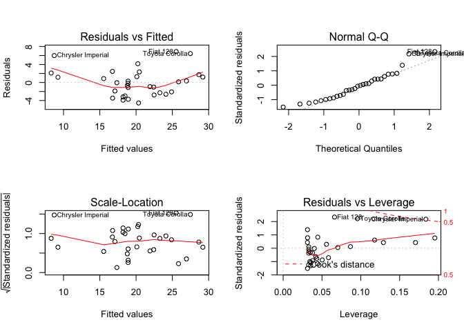
par(mfrow=c(2,2))
plot(fit)

Created on 2020-03-06 by the reprex package (v0.3.0)