verification of adherence of the model to the statistical premises of the least squares method through diagnostic graphs'

[Danilo]

Good morning, I'm new to R and would like to take some questions

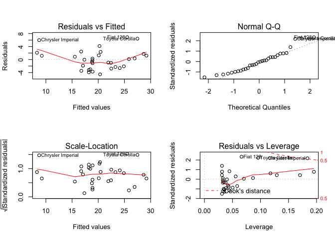
Perform the verification of the model's adherence to the statistical premises of the least squares method through the diagnostic graphs, commenting on the graph of residuals x adjusted values and the graph of the Normal-QQ curve.

how could you do that

[technocrat]

Hi, and welcome!

Please see the FAQ: What's a reproducible example (`reprex`) and how do I create one? Using a reprex, complete with representative data will attract quicker and more answers. Also, if applicable, please see the homework policy.

Let's use mtcars.

fit <- lm(mpg ~ wt, data = mtcars)
summary(fit)
#> 
#> Call:
#> lm(formula = mpg ~ wt, data = mtcars)
#> 
#> Residuals:
#>     Min      1Q  Median      3Q     Max 
#> -4.5432 -2.3647 -0.1252  1.4096  6.8727 
#> 
#> Coefficients:
#>             Estimate Std. Error t value Pr(>|t|)    
#> (Intercept)  37.2851     1.8776  19.858  < 2e-16 ***
#> wt           -5.3445     0.5591  -9.559 1.29e-10 ***
#> ---
#> Signif. codes:  0 '***' 0.001 '**' 0.01 '*' 0.05 '.' 0.1 ' ' 1
#> 
#> Residual standard error: 3.046 on 30 degrees of freedom
#> Multiple R-squared:  0.7528, Adjusted R-squared:  0.7446 
#> F-statistic: 91.38 on 1 and 30 DF,  p-value: 1.294e-10
par(mfrow=c(2,2))
plot(fit)

^{Created on 2020-03-06 by the reprex package (v0.3.0)}