Hello R-community! I am using VAR, I want to forecast how my variable "Arbeidsledighet", which means Unemployement is playing out while having a "shock" in my other variable, "Oljepris" which basically means Oilprice. I understand that I have to use VAR, and impulse response function.
I have this dataset:
> Arbeidsledige_KvartL
# A tibble: 36 x 3
   kvartal    arbeidsledige oljepris
   <date>             <dbl>    <dbl>
 1 2011-03-01         74190    115.
 2 2011-06-01         65487    114.
 3 2011-09-01         65254    113.
 4 2011-12-01         63655    108.
 5 2012-03-01         67669    125.
 6 2012-06-01         64196     95.2
 7 2012-09-01         63060    113.
 8 2012-12-01         62569    108.
 9 2013-03-01         69969    108.
10 2013-06-01         66596    103.
# … with 26 more rows
Then I did:
> attach(Arbeidsledige_KvartL)
> Arbeidsledige=diff(arbeidsledige)
> Oljepris=diff(oljepris)
> arb=cbind(Arbeidsledige, Oljepris)
> library(vars)
> model <- VAR(arb, p = 2, type ="const")
> summary(model)

VAR Estimation Results:
=========================
Endogenous variables: Arbeidsledige, Oljepris
Deterministic variables: const
Sample size: 33
Log Likelihood: -446.499
Roots of the characteristic polynomial:
0.5021 0.1081 0.1081 0.02156
Call:
VAR(y = arb, p = 2, type = "const")


Estimation results for equation Arbeidsledige:
==============================================
Arbeidsledige = Arbeidsledige.l1 + Oljepris.l1 + Arbeidsledige.l2 + Oljepris.l2 + const

                   Estimate Std. Error t value Pr(>|t|)
Arbeidsledige.l1   -0.38853    0.18833  -2.063   0.0485 *
Oljepris.l1      -124.36834   67.41236  -1.845   0.0757 .
Arbeidsledige.l2    0.01194    0.17212   0.069   0.9452
Oljepris.l2       -23.80439   70.60770  -0.337   0.7385
const            -409.51564  775.97023  -0.528   0.6018
---
Signif. codes:  0 ‘***’ 0.001 ‘**’ 0.01 ‘*’ 0.05 ‘.’ 0.1 ‘ ’ 1


Residual standard error: 4296 on 28 degrees of freedom
Multiple R-Squared: 0.2396,	Adjusted R-squared: 0.131
F-statistic: 2.206 on 4 and 28 DF,  p-value: 0.09408


Estimation results for equation Oljepris:
=========================================
Oljepris = Arbeidsledige.l1 + Oljepris.l1 + Arbeidsledige.l2 + Oljepris.l2 + const

                   Estimate Std. Error t value Pr(>|t|)
Arbeidsledige.l1 -3.748e-04  5.339e-04  -0.702    0.488
Oljepris.l1      -2.165e-01  1.911e-01  -1.133    0.267
Arbeidsledige.l2  2.517e-05  4.879e-04   0.052    0.959
Oljepris.l2      -3.958e-02  2.002e-01  -0.198    0.845
const            -1.811e+00  2.200e+00  -0.823    0.417


Residual standard error: 12.18 on 28 degrees of freedom
Multiple R-Squared: 0.06488,	Adjusted R-squared: -0.06871
F-statistic: 0.4856 on 4 and 28 DF,  p-value: 0.7461


Covariance matrix of residuals:
              Arbeidsledige Oljepris
Arbeidsledige      18458084  -6812.8
Oljepris              -6813    148.3

Correlation matrix of residuals:
              Arbeidsledige Oljepris
Arbeidsledige        1.0000  -0.1302
Oljepris            -0.1302   1.0000
Then I tried to plot it, and wanted to forecast how Arbeidsledighet/Unemployement plays out, when Oilprice is going down:
> feir <- irf(model, impulse ="Oljepris", response ="Arbeidsledige", n.ahead = 8, ortho = FALSE, runs = 1000)
> plot(feir)```
Then I got this plot:
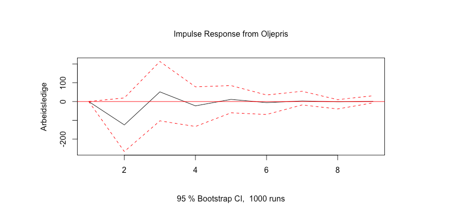
So did I do it right? If not, what should I do, and what did I do wrong? How do I interpret this?