Using R package to implement Bayesian phase I/II dose-finding design for three outcomes

[ran20]

Dear all,

I am trying to implement the work done by Suyu Liu, “A Bayesian Phase I/II Trial Design for Immunotherapy”, using R, since the code attached with that work takes a lot of time (more than 20 hours and the code not complete, I do not know how it produced the tables and the figures).

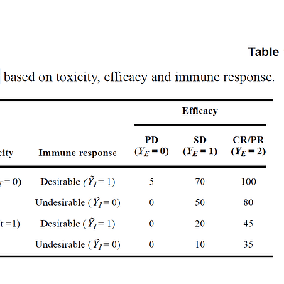
So that I tried to use trialr package trying to get similar or approximate results using the utility functions for sensitivity analysis in table 1 (picture below), but this package allowed me to use just two outcomes ( toxicity, efficacy ) and the work of Liu used three outcomes (immune response, toxicity, and efficacy). I want to see if I used the correct utility (table 1 below) and to see how to add a third outcome ( immune response ) to the model? (Question 1)

I attached to you the code and the output for 50 iterations and 60 patients from the work of Liu and Yuan ( I cannot do more, it took around 12 hours), if you know how he produced the results, (Question 2) I hope you can feed me back.

My goal is : to use their idea to select the best dose in the first stage and to continue in a second stage with only 2 arms clinical trial and the best dose. (may there is another way to do that?)

### My code trying to get similar results using trialr package ###
rm(list = ls())
library(trialr)

 ## Utility from table 1 and Liu and Yuan work.

Uti <- array(0,c(2,3,2)) # order: tox, eff, immuno
Uti[,,1] <- matrix(c(0,0,50,10,80,35),nrow=2)
Uti[,,2] <- matrix(c(5,0,70,20,100,45),nrow=2)

N.max= 60 # patients  

outcomes <- '1NNN 2NNT 3NNT 4NNN 5NTN'
doses = c(.1,.3,.5,.7,.9)


fit <- stan_efftox(outcomes,
                   real_doses =doses,
                   efficacy_hurdle = 0.5, toxicity_hurdle = 0.3,
                   p_e = 0.1, p_t = 0.1,
                   eff0 = 0.5, tox1 = 0.65,
                   eff_star = 0.7, tox_star = 0.25,
                   alpha_mean = -7.9593, alpha_sd = 3.5487,
                   beta_mean = 1.5482, beta_sd = 3.5018,
                   gamma_mean = 0.7367, gamma_sd = 2.5423,
                   zeta_mean = 3.4181, zeta_sd = 2.4406,
                   eta_mean = 0, eta_sd = 0.2,
                   psi_mean = 0, psi_sd = 1,
                   seed = 123)

ndoses <- length(fit$prob_tox)
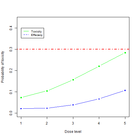
plot(1:ndoses, fit$prob_tox,  type="b", pch=19, xlab="Dose level", ylab="Probability of toxicity", ylim=c(0,max(fit$prob_tox) + 0.15), col="green")
points(1:ndoses,fit$prob_eff,  type="b", pch=18, col="blue")
abline(h=0.3, lwd=2, lty=4, col = "red")
legend(1, 0.4, legend=c("Toxicity", "Effecacy"),
      col=c("green", "blue"), lty=1:2, cex=0.8)

this produce this figure

Thanks in advance