Hello everybody ! I'm currently working on my first RShiny app for financial assets, in order (mainly) to obtain what we call the "Markowitz efficient frontier".
This frontier is the plot representation of all possible efficient "risk/return" combinaison considering given assets (a portfolio). Typically, it's a question of minimization of variance for a given return.
My goal is also to add constraint on my portfolio : thus the subject becomes a question of minimization of variance with constraints. For example, a constraint could be that none of the asset (belonging to the portfolio) weights for less than 2% in the portfolio.
I use the "fPortfolio package" which contains many great tools for this kind of work. When I use this package on a regular R file, it works really fast, even with severals constraints for computing (only 5 to 8 seconds, it depends about the constraint)
However in my Shiny app, the time for ploting the efficient frontier is significantly longer WITHOUT constraints : more than 20 seconds. And if I try to add some constraints, then I don't know how many time it takes : I waited for 10 minutes without getting any plot.
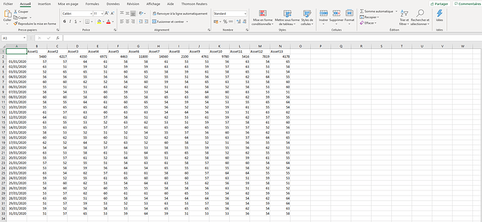
I add my a light version of my app, which contains the problematic lines ; I also a picture of an example of data file that works with the app (it's CSV with yyyy-mm-dd date format). Could please somebody helps me to get faster results for this app ?
It's my first app and I'm also a beginner in programmation so please be indulgent with my synthax ![]() Thanks for reading !
Thanks for reading !
Robin
THE CODE :
packages
library(shiny);library(tidyverse);library(ggplot2);library(plotly);library(corrplot);library(timeSeries);library(fPortfolio);
library(quantmod);library(caTools);library(dplyr);library(PerformanceAnalytics);library(dplyr);library(readr);library(xts);
library(shinydashboard);library(shinyWidgets);library(shinyTime);library(portfolioBacktest);library(graphics)
library(glue);library(profvis);
#######################################UI##################################################
#######################################HEADER
header <- dashboardHeader(title = "Portfolio Analysis")
######################################SIDEBAR
sidebar <- dashboardSidebar(sidebarMenuOutput("menu"),
fileInput('target_upload', 'Numeric data',
accept = c(
'text/csv',
'text/comma-separated-values',
'.csv'
)),
dateRangeInput("dates", h3("Time period"), format = "dd-mm-yyyy",
start = "2020-01-01", end = "2020-01-31" ))
####################################BODY
body <- dashboardBody(tabsetPanel(type = "tabs",
tabPanel("Efficient frontier",
br(),
plotlyOutput("ef"),
br(),
column(3,
h3("Minimum weight for one asset"),
checkboxInput("checkbox_1", "Oui", value = FALSE)),
column(3,numericInput("contrainte_1",h3("Minimum weight for one asset"), value = 0.01, min = 0, max = 1, step = 0.01)))))
ui <- dashboardPage(header, sidebar, body, skin = "red")
server<-function(input,output){![example of data|690x318]
#Function which calls data
df_products_upload <- reactive({
inFile <- input$target_upload
if (is.null(inFile))
return(NULL)
df <- read.csv2(inFile$datapath, header = TRUE,sep = ";")
borne_1<-subset(df, df[,1] == input$dates[1])
borne_2<- subset(df, df[,1] == input$dates[2])
ligne<-as.integer(rownames(borne_1))
lignefin<-as.integer(rownames(borne_2))
df<-df[(1:lignefin),]
if(ligne > 2){
ligne<-ligne-2
for (i in 1:(ligne)){
df<-df[-2,]
}
}
df
})
#Function which computes daily returns
pfRend<-reactive({
df<-df_products_upload()
dftrans<-df[-1,-1]
rownames(dftrans)<-df[-1,1]
df<-dftrans
pfRend<-na.omit(ROC(df, type = "discrete"))
pfRend<-as.timeSeries(pfRend)
pfRend
})
#Function which defines constraints
contraintes <- reactive({
contr<-NULL
contrainte_1<- input$contrainte_1
if(input$checkbox_1 == TRUE){
for (i in 1:13){
newcond<-c(glue("minW[{i}] = {contrainte_1}"))
contr<-cbind(contr,newcond)
contr<-as.character(contr)}
}
else{
contr<-c("LongOnly")
}
return(contr)
})
#Function which computes risk_return
risk_return<-reactive({
pfRend<-pfRend()
spec<-portfolioSpec(
model = list(
type = "MV", optimize = "minRisk",
estimator = "covEstimator", tailRisk = list(),
params = list(alpha = 0.05)),
portfolio = list(
weights = NULL, targetReturn = NULL,
targetRisk = NULL, riskFreeRate = 0, nFrontierPoints =5000,
status = NA),
optim = list(
solver = "solveRquadprog",
objective = c("portfolioObjective", "portfolioReturn", "portfolioRisk"),
options = list(meq = 2), control = list(), trace = FALSE),
messages = list(
messages = FALSE, note = ""),
ampl = list(
ampl = FALSE, project = "ampl", solver = "ipopt",
protocol = FALSE, trace = FALSE)
)
effFrontier <- portfolioFrontier(pfRend, spec, constraint = contraintes())
risk_return<-frontierPoints(effFrontier)
risk_return<-as.data.frame(risk_return)
return(risk_return)
})
plot the efficient frontier
output$ef<-renderPlotly({
p <- ggplot(risk_return(), aes(targetRisk,targetReturn)) + geom_point(colour = "gold")+ expand_limits(x = 0, y = 0) +
labs(title = 'Frontiere efficiente', x = 'Risque', y = 'Esperance de Rendement')+
theme(plot.title = element_text(face = 'bold.italic', hjust = 0.5))
ggplotly(p)
})
}
shinyApp(ui = ui, server = server)
THE DATA :
