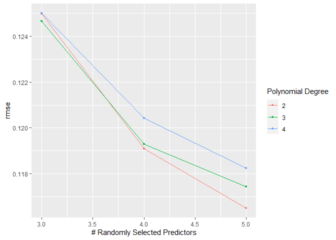
I'm learning tidymodels, and I've been following this blog post. Strangely, I get a different plot when visualizing with autoplot.tune_results() compared to the one on the blog post.
Here's the reprex of the visualization I get:
library(tidymodels)
#> Registered S3 method overwritten by 'tune':
#>   method                   from
#>   required_pkgs.model_spec parsnip
library(doFuture)
#> Loading required package: foreach
#>
#> Attaching package: 'foreach'
#> The following objects are masked from 'package:purrr':
#>
#>     accumulate, when
#> Loading required package: future
library(parallel)

set.seed(1243)

dia_split <- initial_split(diamonds, prop = .1, strata = price)

dia_train <- training(dia_split)
dia_test  <- testing(dia_split)

dia_vfold <- vfold_cv(dia_train, v = 3, repeats = 1, strata = price)

rf_model <-
  rand_forest(mtry = tune()) %>%
  set_mode("regression") %>%
  set_engine("ranger")

dia_rec2 <-
  recipe(price ~ ., data = dia_train) %>%
  step_log(all_outcomes()) %>%
  step_normalize(all_predictors(), -all_nominal()) %>%
  step_dummy(all_nominal()) %>%
  step_poly(carat, degree = tune())

rf_wflow <-
  workflow() %>%
  add_model(rf_model) %>%
  add_recipe(dia_rec2)

rf_param <-
  rf_wflow %>%
  parameters() %>%
  update(mtry = mtry(range = c(3L, 5L)),
         degree = degree_int(range = c(2L, 4L)))

rf_grid <- grid_regular(rf_param, levels = 3)

all_cores <- parallel::detectCores(logical = FALSE) - 1

registerDoFuture()
cl <- makeCluster(all_cores)
plan(future::cluster, workers = cl)

rf_search <- tune_grid(rf_wflow, grid = rf_grid, resamples = dia_vfold,
                       param_info = rf_param)


autoplot(rf_search, metric = "rmse")

Created on 2021-12-21 by the reprex package (v2.0.1.9000)
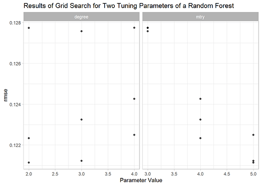
However, the visualization is different on the blog post:
How come the plots are different despite the same code? Is this a matter of version of any of the packages involved?
Thanks.
