Hi,
I'm currently trying to wrap my head around partial dependency plots and i have two questions i was hoping someone could help me with
I have found a number of definitions...
-
"Suppose you would like to understand importance of variable p_i in the model, PDP builds the model averaging other predictor variable except one choosen predictor variable p_i and measures change in response yhat and y, change in response can help identify how a variable is affecting the model" 1
-
"The idea is that the function f(x) tells us how the value of the variable x_j influences the model predictions \hat y after we have “averaged out” the influence of all other variables" 2
-
"The partial dependence plot (short PDP or PD plot) shows the marginal effect one or two features have on the predicted outcome of a machine learning model"3
I think I am getting bogged down in the technical speak about distributions so was hoping to get a layman description of what is happening
From my understanding we take a predictor and change the value of that predictor across a range of values for each row of data. These values are determined by a grid. Depending on the implementation, all other variables are held constant (either at a median or average etc). The mean for all the rows is taken at a single point on the axis. If you plot the individual rows themselves you get an ICE plot. So we see the change in the mean of predictor for all rows in the dataset across a range of pre-determined values and record the model output as that predictor changes. If its a regression problem like the cost of a house, the house price should vary 3. If you get negative values here its because you are getting a result less than the average of the house. If its a classification problem the probability of an instance belonging to a particular class should vary 3.
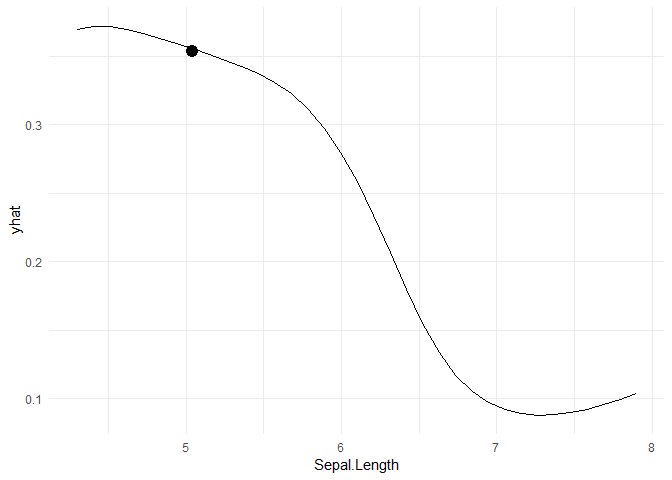
My questions might seem a bit basic but i hope you can help. Taking the example from 4 I replicated the PDP graphs for the Iris dataset to try and predict if a class is setosa or not. I plotted the results and have a point x=5.041176, y = 0.35345465 on the graphs
-
Is my understanding of PDPs above accurate
-
Can someone explain to me what “averaged out” and "marginal distributions" actually mean
-
In relation to my understanding of interpretation, if my sepal length is 5.041176, then the probability that i have a setosa on my hands is on average 35%, all other attributes being held constant
-
At this point
x=5.041176, y = 0.35345465what are all my other attributes held at; for example Sepal.Width, Petal.Length and Petal.Width. Can some one show me a quick calculation in R based on the data?
Thank you very much for your time.
library(tidyverse)
library(e1071)
library(pdp)

mydf <- iris %>%
  mutate(tgt = factor(ifelse(Species == 'setosa', "yes", "no"))) %>%
  select(-Species)

pred.prob <- function(object, newdata) {
  pred <- predict(object, newdata, probability = TRUE)
  prob.setosa <- attr(pred, which = "probabilities")[, "yes"]
  mean(prob.setosa)
}

svm_mod <- svm(tgt ~ ., data = mydf, kernel = "radial", gamma = 0.75,
               cost = 0.25, probability = TRUE)
pdp_graph  <- partial(svm_mod, pred.var = c("Sepal.Length"), probs = TRUE, pred.fun = pred.prob)

ggplot(pdp_graph, aes(x=Sepal.Length, y=yhat)) +
  geom_line() +
  geom_point(x=5.041176, y = 0.35345465, size = 4) +
  theme_minimal()

Created on 2019-03-27 by the reprex package (v0.2.1)