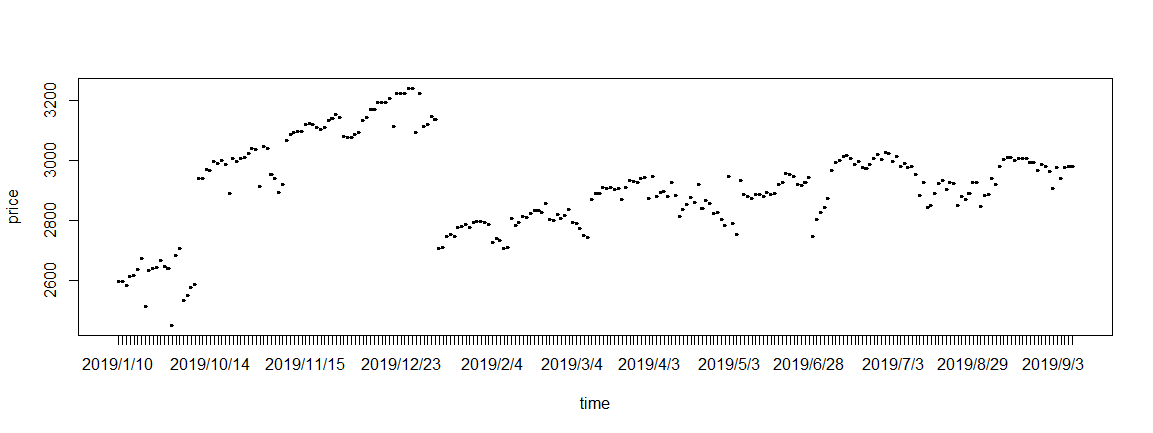
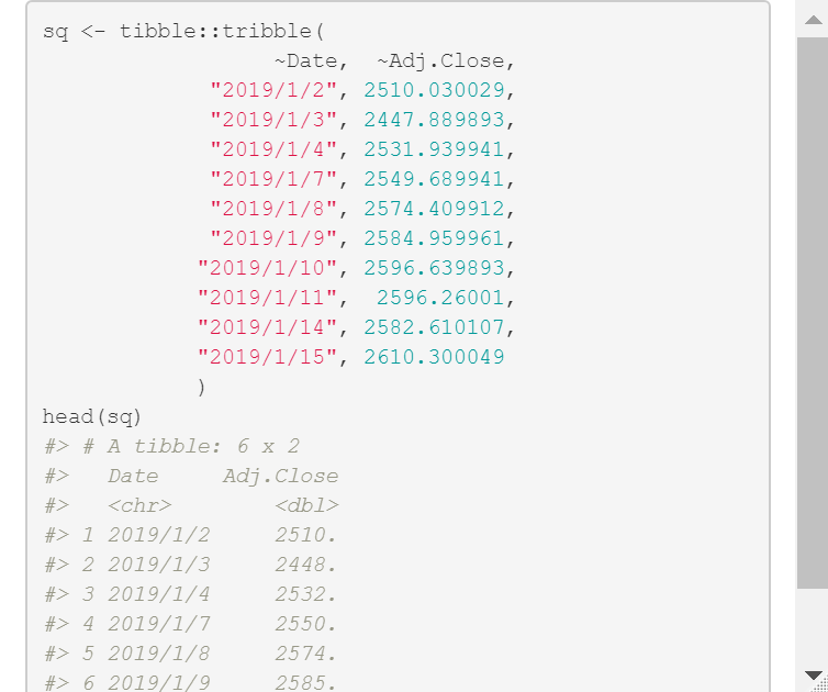
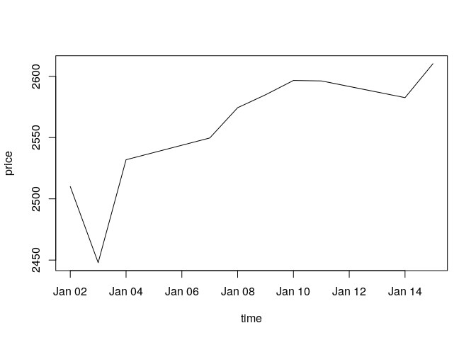
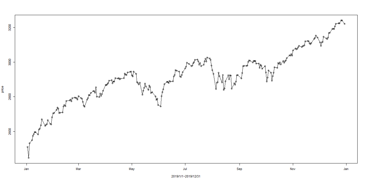
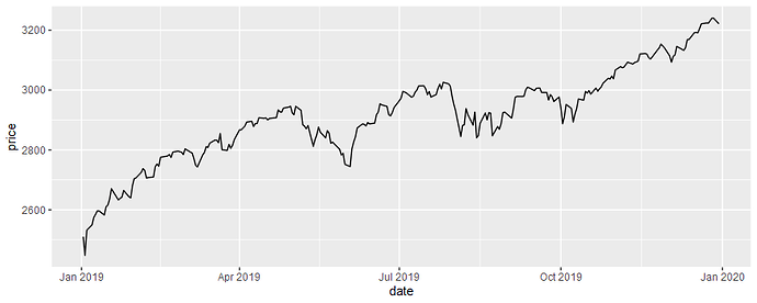
If I understand correctly, your concern is that the x-axis in the new plot seems to have been converted to months, as opposed to dates (yyyy-mm-dd). Correct me if I'm wrong. In that case, this is just due to the data.frame in the reprex example having fewer rows than the data.frame you are using. All of the rows of the reprex data.frame belong to the same year. That's why only months are displayed in the x-axis (years are redundant). Using the data you provided in the a1.pdf file, I put together this code, which should do the job, if I have understoof you correctly. By using ggplot2 to plot the data you have more control over the labels of the x-axis.
library(dplyr)
library(lubridate)
library(ggplot2)
d <- tibble::tribble(
       ~Date.Adj.Close,
    "2019/1/2 2510.03",
    "2019/1/3 2447.89",
    "2019/1/4 2531.94",
    "2019/1/7 2549.69",
    "2019/1/8 2574.41",
    "2019/1/9 2584.96",
   "2019/1/10 2596.64",
   "2019/1/11 2596.26",
   "2019/1/14 2582.61",
    "2019/1/15 2610.3",
    "2019/1/16 2616.1",
   "2019/1/17 2635.96",
   "2019/1/18 2670.71",
    "2019/1/22 2632.9",
    "2019/1/23 2638.7",
   "2019/1/24 2642.33",
   "2019/1/25 2664.76",
   "2019/1/28 2643.85",
      "2019/1/29 2640",
   "2019/1/30 2681.05",
    "2019/1/31 2704.1",
    "2019/2/1 2706.53",
    "2019/2/4 2724.87",
     "2019/2/5 2737.7",
    "2019/2/6 2731.61",
    "2019/2/7 2706.05",
    "2019/2/8 2707.88",
    "2019/2/11 2709.8",
   "2019/2/12 2744.73",
   "2019/2/13 2753.03",
   "2019/2/14 2745.73",
    "2019/2/15 2775.6",
   "2019/2/19 2779.76",
    "2019/2/20 2784.7",
   "2019/2/21 2774.88",
   "2019/2/22 2792.67",
   "2019/2/25 2796.11",
    "2019/2/26 2793.9",
   "2019/2/27 2792.38",
   "2019/2/28 2784.49",
    "2019/3/1 2803.69",
    "2019/3/4 2792.81",
    "2019/3/5 2789.65",
    "2019/3/6 2771.45",
    "2019/3/7 2748.93",
    "2019/3/8 2743.07",
    "2019/3/11 2783.3",
   "2019/3/12 2791.52",
   "2019/3/13 2810.92",
   "2019/3/14 2808.48",
   "2019/3/15 2822.48",
   "2019/3/18 2832.94",
   "2019/3/19 2832.57",
   "2019/3/20 2824.23",
   "2019/3/21 2854.88",
   "2019/3/22 2800.71",
   "2019/3/25 2798.36",
   "2019/3/26 2818.46",
   "2019/3/27 2805.37",
   "2019/3/28 2815.44",
    "2019/3/29 2834.4",
    "2019/4/1 2867.19",
    "2019/4/2 2867.24",
     "2019/4/3 2873.4",
    "2019/4/4 2879.39",
    "2019/4/5 2892.74",
    "2019/4/8 2895.77",
     "2019/4/9 2878.2",
   "2019/4/10 2888.21",
   "2019/4/11 2888.32",
   "2019/4/12 2907.41",
   "2019/4/15 2905.58",
   "2019/4/16 2907.06",
   "2019/4/17 2900.45",
   "2019/4/18 2905.03",
   "2019/4/22 2907.97",
   "2019/4/23 2933.68",
   "2019/4/24 2927.25",
   "2019/4/25 2926.17",
   "2019/4/26 2939.88",
   "2019/4/29 2943.03",
   "2019/4/30 2945.83",
    "2019/5/1 2923.73",
    "2019/5/2 2917.52",
    "2019/5/3 2945.64",
    "2019/5/6 2932.47",
    "2019/5/7 2884.05",
    "2019/5/8 2879.42",
    "2019/5/9 2870.72",
    "2019/5/10 2881.4",
   "2019/5/13 2811.87",
   "2019/5/14 2834.41",
   "2019/5/15 2850.96",
   "2019/5/16 2876.32",
   "2019/5/17 2859.53",
   "2019/5/20 2840.23",
   "2019/5/21 2864.36",
   "2019/5/22 2856.27",
   "2019/5/23 2822.24",
   "2019/5/24 2826.06",
   "2019/5/28 2802.39",
   "2019/5/29 2783.02",
   "2019/5/30 2788.86",
   "2019/5/31 2752.06",
    "2019/6/3 2744.45",
    "2019/6/4 2803.27",
    "2019/6/5 2826.15",
    "2019/6/6 2843.49",
    "2019/6/7 2873.34",
   "2019/6/10 2886.73",
   "2019/6/11 2885.72",
   "2019/6/12 2879.84",
   "2019/6/13 2891.64",
   "2019/6/14 2886.98",
   "2019/6/17 2889.67",
   "2019/6/18 2917.75",
   "2019/6/19 2926.46",
   "2019/6/20 2954.18",
   "2019/6/21 2950.46",
   "2019/6/24 2945.35",
   "2019/6/25 2917.38",
   "2019/6/26 2913.78",
   "2019/6/27 2924.92",
   "2019/6/28 2941.76",
    "2019/7/1 2964.33",
    "2019/7/2 2973.01",
    "2019/7/3 2995.82",
    "2019/7/5 2990.41",
    "2019/7/8 2975.95",
    "2019/7/9 2979.63",
   "2019/7/10 2993.07",
   "2019/7/11 2999.91",
   "2019/7/12 3013.77",
    "2019/7/15 3014.3",
   "2019/7/16 3004.04",
   "2019/7/17 2984.42",
   "2019/7/18 2995.11",
   "2019/7/19 2976.61",
   "2019/7/22 2985.03",
   "2019/7/23 3005.47",
   "2019/7/24 3019.56",
   "2019/7/25 3003.67",
   "2019/7/26 3025.86",
   "2019/7/29 3020.97",
   "2019/7/30 3013.18",
   "2019/7/31 2980.38",
    "2019/8/1 2953.56",
    "2019/8/2 2932.05",
    "2019/8/5 2844.74",
    "2019/8/6 2881.77",
    "2019/8/7 2883.98",
    "2019/8/8 2938.09",
    "2019/8/9 2918.65",
    "2019/8/12 2882.7",
   "2019/8/13 2926.32",
    "2019/8/14 2840.6",
    "2019/8/15 2847.6",
   "2019/8/16 2888.68",
   "2019/8/19 2923.65",
   "2019/8/20 2900.51",
   "2019/8/21 2924.43",
   "2019/8/22 2922.95",
   "2019/8/23 2847.11",
   "2019/8/26 2878.38",
   "2019/8/27 2869.16",
   "2019/8/28 2887.94",
   "2019/8/29 2924.58",
   "2019/8/30 2926.46",
    "2019/9/3 2906.27",
    "2019/9/4 2937.78",
       "2019/9/5 2976",
    "2019/9/6 2978.71",
    "2019/9/9 2978.43",
   "2019/9/10 2979.39",
   "2019/9/11 3000.93",
   "2019/9/12 3009.57",
   "2019/9/13 3007.39",
   "2019/9/16 2997.96",
    "2019/9/17 3005.7",
   "2019/9/18 3006.73",
   "2019/9/19 3006.79",
   "2019/9/20 2992.07",
   "2019/9/23 2991.78",
    "2019/9/24 2966.6",
   "2019/9/25 2984.87",
   "2019/9/26 2977.62",
   "2019/9/27 2961.79",
   "2019/9/30 2976.74",
   "2019/10/1 2940.25",
   "2019/10/2 2887.61",
   "2019/10/3 2910.63",
   "2019/10/4 2952.01",
   "2019/10/7 2938.79",
   "2019/10/8 2893.06",
    "2019/10/9 2919.4",
  "2019/10/10 2938.13",
  "2019/10/11 2970.27",
  "2019/10/14 2966.15",
  "2019/10/15 2995.68",
  "2019/10/16 2989.69",
  "2019/10/17 2997.95",
   "2019/10/18 2986.2",
  "2019/10/21 3006.72",
  "2019/10/22 2995.99",
  "2019/10/23 3004.52",
  "2019/10/24 3010.29",
  "2019/10/25 3022.55",
  "2019/10/28 3039.42",
  "2019/10/29 3036.89",
  "2019/10/30 3046.77",
  "2019/10/31 3037.56",
   "2019/11/1 3066.91",
   "2019/11/4 3078.27",
   "2019/11/5 3074.62",
   "2019/11/6 3076.78",
   "2019/11/7 3085.18",
   "2019/11/8 3093.08",
  "2019/11/11 3087.01",
  "2019/11/12 3091.84",
  "2019/11/13 3094.04",
  "2019/11/14 3096.63",
  "2019/11/15 3120.46",
  "2019/11/18 3122.03",
  "2019/11/19 3120.18",
  "2019/11/20 3108.46",
  "2019/11/21 3103.54",
  "2019/11/22 3110.29",
  "2019/11/25 3133.64",
  "2019/11/26 3140.52",
  "2019/11/27 3153.63",
  "2019/11/29 3140.98",
   "2019/12/2 3113.87",
    "2019/12/3 3093.2",
   "2019/12/4 3112.76",
   "2019/12/5 3117.43",
   "2019/12/6 3145.91",
   "2019/12/9 3135.96",
  "2019/12/10 3132.52",
  "2019/12/11 3141.63",
  "2019/12/12 3168.57",
   "2019/12/13 3168.8",
  "2019/12/16 3191.45",
  "2019/12/17 3192.52",
  "2019/12/18 3191.14",
  "2019/12/19 3205.37",
  "2019/12/20 3221.22",
  "2019/12/23 3224.01",
  "2019/12/24 3223.38",
  "2019/12/26 3239.91",
  "2019/12/27 3240.02",
  "2019/12/30 3221.29"
  ) %>%
  separate(Date.Adj.Close, c("date", "price"), sep = " ") %>%
  mutate(date = ymd(date),
         price = as.numeric(price))

ggplot(d, aes(x = date,  y = price)) +
  geom_line()
