Understanding arguments to functions is something that I had a lot of trouble with (and shouldn't have in retrospect).
One of the hard things to get used to in R is the concept that everything is an object that has properties. Some objects have properties that allow them to operate on other objects to produce new objects. Those are functions.
Think of R as school algebra writ large: f(x) = y, where the objects are f, a function, x, an object (and there may be several) termed the argument and y is an object termed a value, which can be as simple as a single number (aka an atomic vector) or a very packed object with a multitude of data and labels.
And, because functions are also objects, they can be arguments to other functions, like the old g(f(x)) = y. (Trivia, this is called being a first class object.)
Although there are function objects in R that operate like control statements in imperative/procedural language, they are best used "under the hood." As it presents to users interactively, R is a functional programming language. Instead of saying
take this, take that, do this, then do that, then if the result is this one thing, do this other thing, but if not do something else and give me the answer
in the style of most common programming languages. However, R allows the user to say
use this function to take this argument and turn it into the value I want for a result
Every function has a signature
pmap_dbl(.l, .f, ...)
The first, .l, is a
.l A list of vectors, such as a data frame. The length of .l determines the number of arguments that .f will be called with. List names will be used if present.
.f A function, formula, or vector (not necessarily atomic).
\cdots If a formula, e.g. ~ .x + 2, it is converted to a function
for more arguments, use ..1, ..2, ..3 etc
Breaking down
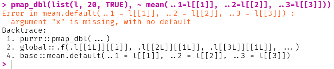
pmap_dbl(list(l, 20, TRUE), ~ mean(..1, ..2, ..3))
\ldots is represented by list(l, 20, TRUE) as .l and ~ mean(..1, ..2, ..3)) as .f. What does it do?
Let's take the .l argument first.
str(list(l, 20, TRUE))
List of 3
 $ :List of 3
  ..$ : num [1:10] -0.638 -0.287 1.057 -2.519 -1.835 ...
  ..$ : num [1:100] -0.456 1.446 0.448 0.855 -0.106 ...
  ..$ : num [1:1000] 0.159 0.573 0.587 -0.267 0.352 ...
 $ : num 20
 $ : logi TRUE
It's a list with a list of three elements, 20 and TRUE. The list within the list is a list of lists.
str(l)
List of 3
 $ : num [1:10] -0.638 -0.287 1.057 -2.519 -1.835 ...
 $ : num [1:100] -0.456 1.446 0.448 0.855 -0.106 ...
 $ : num [1:1000] 0.159 0.573 0.587 -0.267 0.352 ...
each of those is aso a list
 str(l[1])
List of 1
 $ : num [1:10] -0.638 -0.287 1.057 -2.519 -1.835 ...
We're now almost down to something we can take a mean of.
mean(l[[1]])
[1] -0.6441985
But that's not the argument to pmap_dbl that's being used
mean(c(l[[1]],20,TRUE))
[1] 1.213168
which is nicely abbreviated by ..1.
This is a long-winded way of saying that objects in R can easily go very deep, and it pays to take a pause to do this knd of anlaysis.