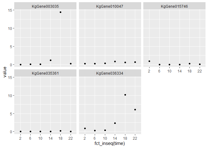
I have a large RNA-seq dataset but it is badly formatted so that the column titles contain too much information (times and multiple conditions i.e. Leaf Pair 1/2, 2am, Well-Watered).
I have used Filter to identify some interesting candidate genes however, I now want to plot these candidate genes to further analyse them. But there are hundreds of potential genes and doing this manually would be a massive time consumer.
I want to use R studio to create a way that I can do this in a bit less time.
I thought I could do this by creating a few vectors and creating a new matrix for each gene - still time consuming but hopefully easier once I have done it once.
My plan was to create a time vector e.g. Time <- c(2, 6, 10, 14, 18, 22).
This would be followed by several vectors representing the different conditions (LP1/2 WW, LP1/2 Droughted, etc) however, I'm finding this v difficult.
Code tried:
Time <- c(2,6,10,14,18,22)
LP1_2.WW <- c(KG$LP1_2.2.WW["KgGene009244"],
              KG$LP1_2.6.WW["KgGene009244"],
              KG$LP1_2.10.WW["KgGene009244"],
              KG$LP1_2.14.WW["KgGene009244"],
              KG$LP1_2.18.WW["KgGene009244"],
              KG$LP1_2.22.WW["KgGene009244"])
I thought this had worked but it gave me this:
LP1_2.WW
[1] NA NA NA NA NA NA
Can anyone give me any advice in regard to this problem?
Edit. This is a small representation of my data to help (thanks siddharthprabhu):
gene_id  LP1_2.2.WW LP1_2.6.WW LP1_2.10.WW
1 KgGene035361 0.009642409 0.04449862  0.01424170
2 KgGene003035 0.000000000 0.02175135  0.02393138
3 KgGene036334 0.901683359 0.33820539  0.41184255
4 KgGene010047 0.254509323 0.19999860  0.36083751
5 KgGene015746 0.917772167 0.00000000  0.00000000
  LP1_2.14.WW LP1_2.18.WW LP1_2.22.WW
1   0.0000000   0.1913271  0.00000000
2   1.2104296  14.4373827  0.19946812
3   2.3094718  10.1677683  6.05295979
4   0.8071359   0.5446581  0.62771431
5   0.0000000   0.2677535  0.03470217
>
Edit: I would want to make some line graphs with this data. This is the script I've written so far:
#Create the individual vectors containing the values for Time and the diff conditions####

Time <- c(2,6,10,14,18,22)
LP1_2.WW <- c(KG$LP1_2.2.WW["KgGene009244"],
              KG$LP1_2.6.WW["KgGene009244"],
              KG$LP1_2.10.WW["KgGene009244"],
              KG$LP1_2.14.WW["KgGene009244"],
              KG$LP1_2.18.WW["KgGene009244"],
              KG$LP1_2.22.WW["KgGene009244"])
LP1_2.D<-c(KG$LP1_2.2.D["KgGene009244"],
           KG$LP1_2.6.D["KgGene009244"],
           KG$LP1_2.10.D["KgGene009244"],
           KG$LP1_2.14.D["KgGene009244"],
           KG$LP1_2.18.D["KgGene009244"],
           KG$LP1_2.22.D["KgGene009244"])
LP3_5.WW<-c(KG$LP3_5.2.WW["KgGene009244"],
            KG$LP3_5.6.WW["KgGene009244"],
            KG$LP3_5.10.WW["KgGene009244"],
            KG$LP3_5.14.WW["KgGene009244"],
            KG$LP3_5.18.WW["KgGene009244"],
            KG$LP3_5.22.WW["KgGene009244"])
LP3_5.D<-c(KG$LP3_5.2.D["KgGene009244"],
           KG$LP3_5.6.D["KgGene009244"],
           KG$LP3_5.10.D["KgGene009244"],
           KG$LP3_5.14.D["KgGene009244"],
           KG$LP3_5.18.D["KgGene009244"],
           KG$LP3_5.22.D["KgGene009244"])


#Combine vectors into a matrix to plot the gene expression####

GraphingMatrix<-cbind(Time, LP1_2.WW, LP1_2.D, LP3_5.WW, LP3_5.D)

#Plot this data####

min_value = min(GraphingMatrix[,2:ncol(GraphingMatrix)])
max_value = max(GraphingMatrix[,2:ncol(GraphingMatrix)])

plot(x=GraphingMatrix$Time, y=GraphingMatrix$LP1_2.WW, type='l', ylim=c(min_value, max_value), col='green')
lines(x=GraphingMatrix$Time, y=GraphingMatrix$LP1_2.D, col='red')
lines(x=GraphingMatrix$Time, y=GraphingMatrix$LP3_5.WW, col='blue')
lines(x=GraphingMatrix$Time, y=GraphingMatrix$LP3_5.D, col='orange')
legend(x = 'topright',
       legend=c('LP1_2.WW','LP1_2.D','LP3_5.WW','LP3_5.D'),
       col=c('green','red','blue','orange'),
       lty = 1, lwd = 1.5)

#ggplot2 of the data ####

KG_Graphing_melt <- melt(GraphingMatrix, id.vars = "Time")
head(KG_Graphing_melt)

colnames(KG_Graphing_melt) <- c("Time", "Leaf Pair and Condition")
l1<-ggplot(KG_Graphing_melt,aes(x=Time,y=Expression))+
  geom_point(aes(colour=Condition))+geom_line(aes(colour=Condition))+
  theme_bw(base_size=16)+
  theme(legend.position = "right")
