Trying to arrange plots in ggarrange

[ctheisen]

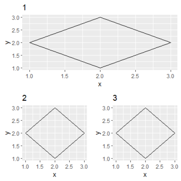
So I have three plots (information on these below) and I want to arrange them so that the first plot is the only one in the first row, and the other two are in the bottom row, and then try to scale them to fit everything in a readable format.

data:

> head(dat.light)
# A tibble: 6 × 4
  title                                                         Role                     sample             value
  <chr>                                                         <chr>                    <chr>              <dbl>
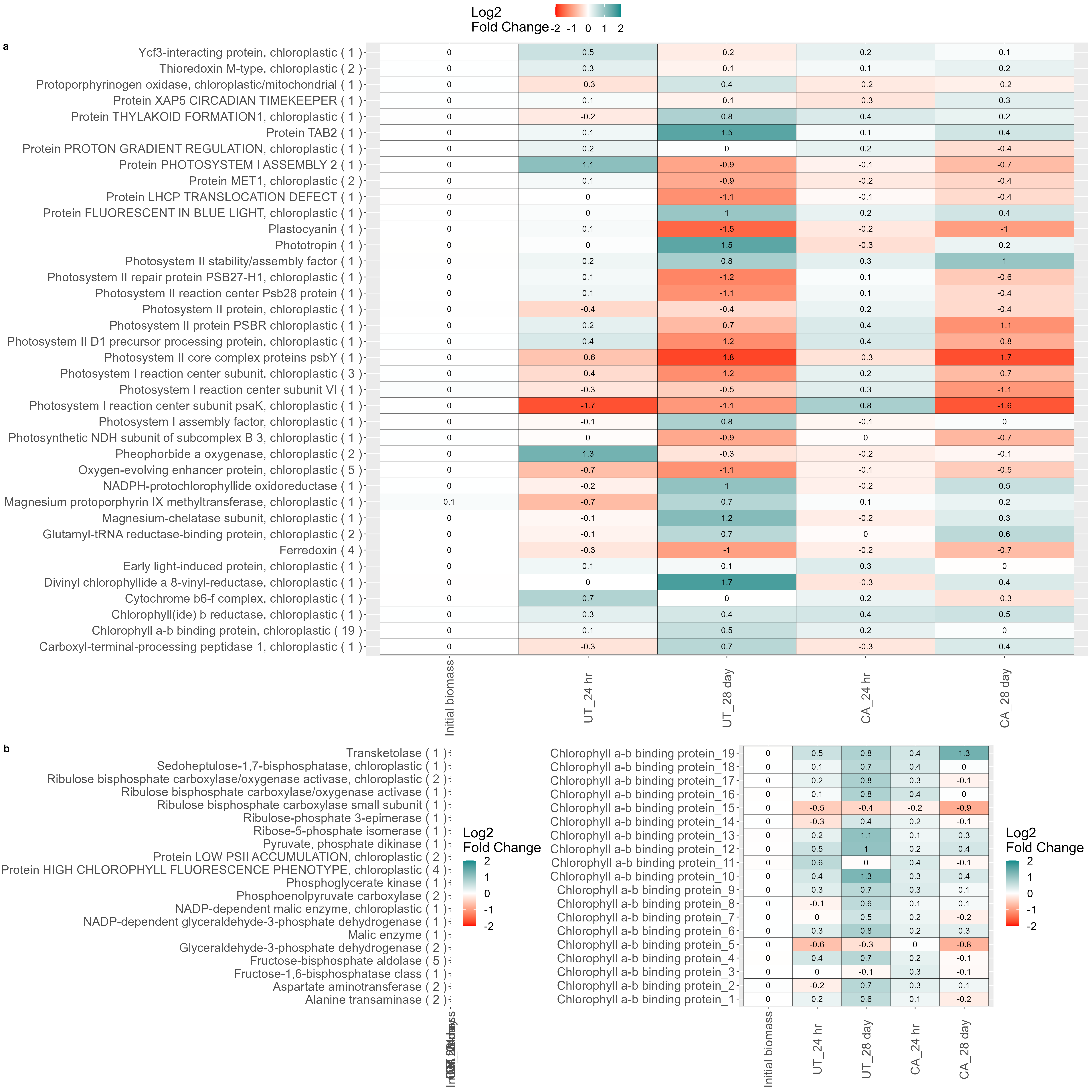
1 Carboxyl-terminal-processing peptidase 1, chloroplastic ( 1 ) PSII processing          Initial biomass -0.00215
2 Carboxyl-terminal-processing peptidase 1, chloroplastic ( 1 ) PSII processing          UT_24 hr        -0.282  
3 Carboxyl-terminal-processing peptidase 1, chloroplastic ( 1 ) PSII processing          UT_28 day        0.676  
4 Carboxyl-terminal-processing peptidase 1, chloroplastic ( 1 ) PSII processing          CA_24 hr        -0.256  
5 Carboxyl-terminal-processing peptidase 1, chloroplastic ( 1 ) PSII processing          CA_28 day        0.358  
6 Chlorophyll a-b binding protein, chloroplastic ( 19 )         Light-Harvesting Complex Initial biomass -0.00148
> head(dat.dark)
# A tibble: 6 × 4
  title                                                                Role          sample            value
  <chr>                                                                <chr>         <chr>             <dbl>
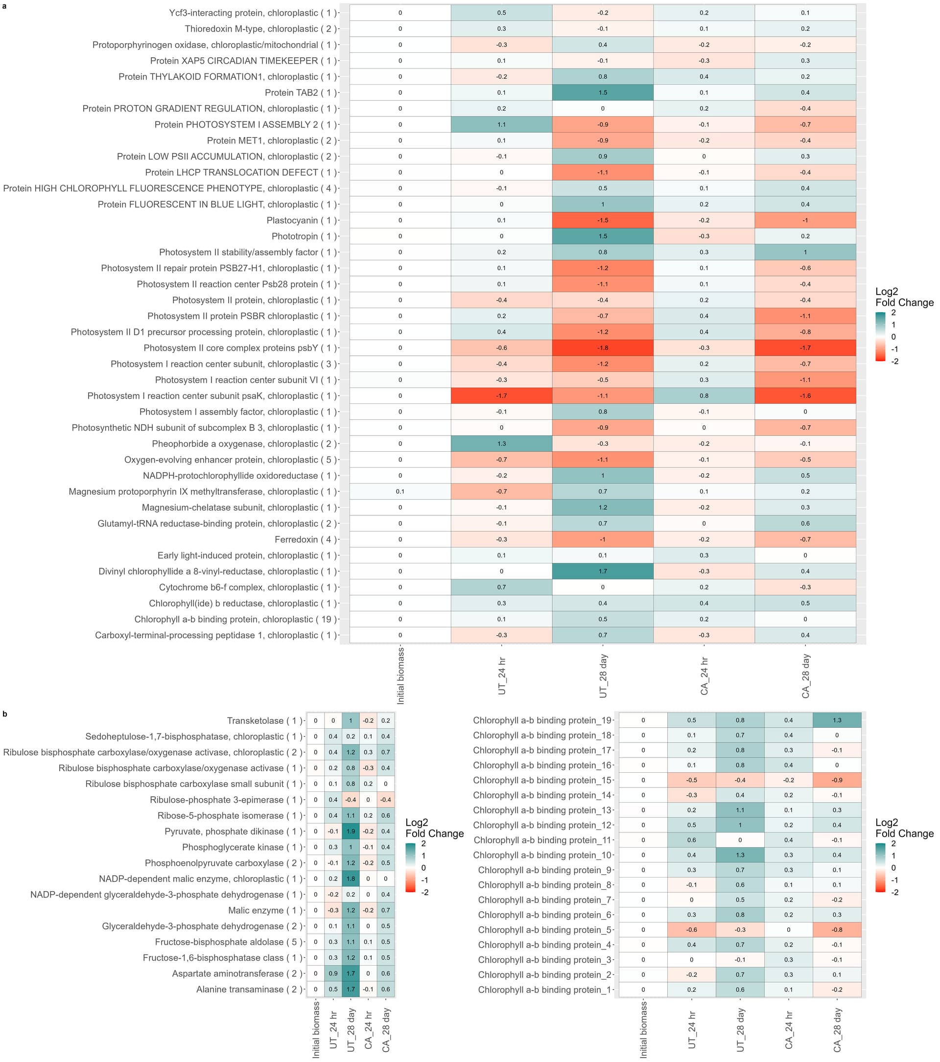
1 Protein HIGH CHLOROPHYLL FLUORESCENCE PHENOTYPE, chloroplastic ( 4 ) PSII Assembly Initial biomass  0.0085
2 Protein HIGH CHLOROPHYLL FLUORESCENCE PHENOTYPE, chloroplastic ( 4 ) PSII Assembly UT_24 hr        -0.0875
3 Protein HIGH CHLOROPHYLL FLUORESCENCE PHENOTYPE, chloroplastic ( 4 ) PSII Assembly UT_28 day        0.484 
4 Protein HIGH CHLOROPHYLL FLUORESCENCE PHENOTYPE, chloroplastic ( 4 ) PSII Assembly CA_24 hr         0.0676
5 Protein HIGH CHLOROPHYLL FLUORESCENCE PHENOTYPE, chloroplastic ( 4 ) PSII Assembly CA_28 day        0.441 
6 Protein LOW PSII ACCUMULATION, chloroplastic ( 2 )                   PSII Assembly Initial biomass -0.0006
> head(cbp_longer)
# A tibble: 6 × 3
  Protein                           sample             value
  <chr>                             <chr>              <dbl>
1 Chlorophyll a-b binding protein_1 Initial biomass -0.00125
2 Chlorophyll a-b binding protein_1 UT_24 hr         0.198  
3 Chlorophyll a-b binding protein_1 UT_28 day        0.599  
4 Chlorophyll a-b binding protein_1 CA_24 hr         0.148  
5 Chlorophyll a-b binding protein_1 CA_28 day       -0.193  
6 Chlorophyll a-b binding protein_2 Initial biomass  0.016  

Code for plots;

plot_light<-ggplot(dat.light, aes(x = factor(sample,level=level_order), y=title,fill=value)) +
  geom_tile(color = "black")+
  scale_fill_gradient2(limits=c(-2,2),low = "red",
                       mid = "white",
                       high = "cyan4")+
  guides(fill=guide_colourbar(title='Log2 \nFold Change'))+
  theme(text=element_text(size=18),axis.text=element_text(size=16),axis.text.x=element_text(angle=90,vjust=0.5),axis.title=element_blank(),plot.title=element_text(size=18,hjust=0.5))+
  geom_text(aes(label=round(value,1)))

photo_dark<-ggplot(dat.dark, aes(x = factor(sample,level=level_order), y=title,fill=value)) +
  geom_tile(color = "black")+
  scale_fill_gradient2(limits=c(-2,2),low = "red",
                       mid = "white",
                       high = "cyan4")+
  # coord_fixed(ratio=0.2)+
  guides(fill=guide_colourbar(title='Log2 \nFold Change'))+
  theme(text=element_text(size=18),axis.text=element_text(size=16),axis.text.x=element_text(angle=90,vjust=0.5),axis.title=element_blank(),plot.title=element_text(size=18,hjust=0.5))+
  geom_text(aes(label=round(value,1)))

cbp_plot<-ggplot(cbp_longer, aes(x = factor(sample,level=level_order), y=factor(Protein,level=prot_level),fill=value)) +
  geom_tile(color = "black")+
  scale_fill_gradient2(limits=c(-2,2),low = "red",
                       mid = "white",
                       high = "cyan4")+
  guides(fill=guide_colourbar(title='Log2 \nFold Change'))+
  theme(text=element_text(size=18),axis.text=element_text(size=16),axis.text.x=element_text(angle=90,vjust=0.5),axis.title=element_blank(),plot.title=element_text(size=18,hjust=0.5))+
  geom_text(aes(label=round(value,1)))

I'm using ggarrange() to try to format them, but I can't figure out how to get the photo_light centered and alone in the first row, and put the other two on the bottom row. Also, any tips on formatting for these is greatly appreciated as this is new to me.

ggarrange(plot_light,photo_dark,cbp_plot,ncol=2,nrow=2,heights=c(2,0.7),labels="auto",common.legend=TRUE)

[nirgrahamuk]

use a nesting approach; i.e.
a ggarrange that is 1 row and 2 cols ; with those plots.
Then a ggarrange with 2 rows and 1 col; where the first row is your top chart; and the bottom row is the prior ggarrange you made.

[ctheisen]

Can you help me figure out what that looks like?

Do you mean something like this?

``r
ggarrange(plot_light,photo_dark,cbp_plot,nrow=1,ncol=2,ggarrange(nrow=2,ncol=1))

[nirgrahamuk]

library(ggplot2)

# Create data for the letter A
diamond_shape <- data.frame(x = c(1, 2, 3, 2, 1), 
                       y = c(2, 3, 2, 1, 2))

# Create the ggplot chart
p1 <- p2 <- p3 <- ggplot(diamond_shape, aes(x, y)) + 
  geom_path()

# label so we can differentiate them easily
p1 <- p1 + ggtitle("1")
p2 <- p2 + ggtitle("2")
p3 <- p3 + ggtitle("3")

library(ggpubr)

bottom_row <- ggarrange(p2,p3, ncol=2,nrow=1)

ggarrange(p1,bottom_row,ncol=1,nrow=2)

[ctheisen]

Ah, so that's a start, but now my top figure is huge and some of the bottom figures are cut, as shown in the figure. Is there a way to then scale the top row so it's smaller and centered above the others?

[nirgrahamuk]

from ?ggarrange

widths	
(optional) numerical vector of relative columns widths. For example, in a two-column grid, widths = c(2, 1) would make the first column twice as wide as the second column.

heights	
same as widths but for column heights.

Therefore

ggarrange(p1,bottom_row,ncol=1,nrow=2,heights = c(1,2))

would make the bottom row twice the height of the top row

[ctheisen]

So I adjusted the height, and that works fine, but I am also trying to narrow the top figure only, so I used widths (0.5,1), but it isn't scaling this first figure widthwise. As shown in these examples, both figures look the same.

bottom_row<-ggarrange(photo_dark,cbp_plot,ncol=2,nrow=1)
ggarrange(plot_light,bottom_row,ncol=1,nrow=2,heights=c(2,1),widths=c(0.5,1),labels="auto")

ggarrange(plot_light,bottom_row,ncol=1,nrow=2,heights=c(2,1),widths=c(1,0.5),labels="auto")

[nirgrahamuk]

Probably a convenient way is to make a top row, of 3 columns the centre with your plot the others with blank plots, and adjust the relative widths of those 3.
It wont do anyhting to adjust widths on your final plot as its one of only one column...