Tidy data: One standard or two?

I am confused about some aspects of the definition of tidy data, particularly as applied to time series. Suppose I have observation of a number of different variables for each period. Usually I would think of this as a rectangular array, with the first value probably a date, an observation number, or some other unique identifier, and the other variables in columns. That seems to correspond to the definition of a tidy data set, with one column for each variable.

But it seems like for a lot of purposes, especially with respect to graphing with ggplot, it is preferable to use “long format,” where all the variable values are in a single column and we have a column for value type with n values, in place of n distinct variables in n columns.

What is confusing me is that Hadley has stated in several places that tidy data constitutes a way of putting all your data into a unique standardized format. That makes me think that one of these formats is not considered tidy. Based on his expository definitions, I’d say the wide format was the tidy one. But when I look at the format that is easiest to use with several tidyverse tools, I’d say it was the narrow format. That is not always true – purrr, for example, seems to prefer a wide format as a way of organizing the subsets of your data that it acts on – but it is often true.

To me, it seems that this ambiguity is potentially troubling, especially as more and more people are writing packages based on data manipulation procedures advertised as tidy. Are there two tidy standards, or just one?

I’d welcome any clarifying thoughts on this.

1 Like

Great question to promote clear thinking.

Based on my time series experience, my possibly fuzzy understanding is that each time increment is an observation of one or more variables.

The x-axis is the value of the time increment, and the y-axis is one or more layers with the related variable values.

There is not a single, unique definition as to what is tidy. As a general rule, each row should be a unique observation. However, your unit of observation may differ for different analyses. I might want to answer a question for which the correct unit of observation is a unique patient. I might later want to answer a different question for which the correct unit of observation is a unique patient encounter. In the second case, each patient will appear multiple times in a taller dataset. In each case, the data are tidy, in that there is only one observation per row, but the unit of observation has changed.
Most of the time, tidying a dataset means that we will make it taller. In part, this is because most people faced with a blank spreadsheet will enter their data for their first observations in a single column, then, for subsequent observations, will add new columns from left to right. The tidyr package gives us tools to tidy this common data issue, usually with pivot_longer.

6 Likes

Thanks for your thoughts, technocrat. I agree that one observation per period is the common intuitive way of arranging time series, unless the data is panel-like.

But it is really hard to graph the data like that in ggplot. It becomes easy if instead you have a factor column for variable type (gdp, population, etc.), and a date column a column for all the data, and a date column. You need an explicit date column in this long-form representation because the data will recur once for each variable.

However, I think it worth observing that the architecture of ggplot was designed before the tidy data concept was clearly enunciated. I am hoping that more experienced programmers can tell me whether, once we move on to explicitly tidy functional design, this three column long format remains the preferred, or easiest, or most-tidy way of arranging data. When I think about dplyr functions, for instance, it seems like the "one column per variable type" representation is more natural and "tidier." But I am not sure I am right about this.

1 Like

Thanks, phiggins! I quite agree that a single underlying data set data set may support multiple data structures with different units of observation. But this is not the focus of my question. Every time series data set with multiple variables can be represented in a wide "one column per variable" format, or in a three-column long format with a date column, a variable type column, and a data column. See my reply to technocrat for a more complete discussion. My question is: Should the three-column long format always be preferred, or should the column-for-each-variable format be preferred for all purposes other than graphing with the ggplot family of of packages? Or is there some other dividing line I haven't thought of?

Could we reify the discussion with a reproducible example, called a reprex?

Sure, technocrat.

yr. <- 1990:1995
nm. <- runif(6)
tx. <- letters[1:6]
fc. <- paste0(tx., round(nm. * 100, 0))

Note: My "." suffixes, inspired by Hadley's . prefixes, are just a way of
making short words that are often already functions or variables into my own
unique variable or function names. They have no meaning beyond that.'

tb_wide <- tibble(year. = yr., num. = nm., txt. = tx., fact. = fc.) # , key = year., index = year.)
tb_wide

A tibble: 6 x 4
year. num. txt. fact.

1 1990 0.642 a a64
2 1991 0.876 b b88
3 1992 0.779 c c78
4 1993 0.797 d d80
5 1994 0.455 e e46
6 1995 0.410 f f41

tb_long <- tb_wide %>%

  • mutate(num_t = as.character(num.), num. = NULL) %>%
    Because you can not put numeric and character values in the same vector. (These are vctrs-style
    vectors and vec_c produces errors for mismatched types, rather than base c's coersion).
  • pivot_longer(-year., names_to = "var_name", values_to = "value")

tb_long

A tibble: 18 x 3
year. var_name value

1 1990 txt. a
2 1990 fact. a64
3 1990 num_t 0.642288258532062
4 1991 txt. b
5 1991 fact. b88
6 1991 num_t 0.876269212691113
7 1992 txt. c
8 1992 fact. c78
9 1992 num_t 0.778914677444845
10 1993 txt. d
11 1993 fact. d80
12 1993 num_t 0.79730882588774
13 1994 txt. e
14 1994 fact. e46
15 1994 num_t 0.455274453619495
16 1995 txt. f
17 1995 fact. f41
18 1995 num_t 0.410084082046524

ts_long <- as_tsibble(tb_long, index = year., key = var_name)
ts_long

A tsibble: 18 x 3 [1Y]
Key: var_name [3]
year. var_name value

1 1990 fact. a64
2 1991 fact. b88
3 1992 fact. c78
4 1993 fact. d80
5 1994 fact. e46
6 1995 fact. f41
7 1990 num_t 0.642288258532062
8 1991 num_t 0.876269212691113
9 1992 num_t 0.778914677444845
10 1993 num_t 0.79730882588774
11 1994 num_t 0.455274453619495
12 1995 num_t 0.410084082046524
13 1990 txt. a
14 1991 txt. b
15 1992 txt. c
16 1993 txt. d
17 1994 txt. e
18 1995 txt. f

You can not do this with the wide format, I'm pretty sure, because there is no
way to specify the key to uniquely identify each time/variable combination
when there are multiple variables on one row.

For a countervailing argument, the vctrs rules seem designed to discourage
long formats like this, since values in the value column are neither coerced
to a common type nor allowed to have different types. I don't see any way
that tsibble can handle numeric and non-numeric values in the same dataset.

tsibble does

I still don't understand how the formatting rules here differ from stackoverflow. My apologies.

1 Like

Here is how

Thanks for making the issue more concrete for me, @andrewH.

I'll begin with the Gospel of @hadley in #RForDataScientists, using the via negativa in R for Data Science

Before we continue on to other topics, it’s worth talking briefly about non-tidy data. Earlier in the chapter, I used the pejorative term “messy” to refer to non-tidy data. That’s an oversimplification: there are lots of useful and well-founded data structures that are not tidy data. There are two main reasons to use other data structures:
Alternative representations may have substantial performance or space advantages.
Specialised fields have evolved their own conventions for storing data that may be quite different to the conventions of tidy data.
Either of these reasons means you’ll need something other than a tibble (or data frame). If your data does fit naturally into a rectangular structure composed of observations and variables, I think tidy data should be your default choice. But there are good reasons to use other structures; tidy data is not the only way.
If you’d like to learn more about non-tidy data, I’d highly recommend this thoughtful blog post by Jeff Leek

Taking the Nicosian Creed approach of what does constitute tidy, from the same Gospel

There are three interrelated rules which make a dataset tidy:
Each variable must have its own column.
Each observation must have its own row.
Each value must have its own cell.

The key definition (forgive me my sins, for I came here originally from the law) is observation, which I can't find in the online version

An observation, or a case, is a set [emphasis added] of measurements under similar conditions (you usually make all of the measures in an observation at the same time [emphasis added] and on the same object [emphasis added]. An observation will contain several values, each associated with a different variable ... [or] a data point.

Therefore, I think, there is no inconsistency between "tidy" and `a rectangular array, with the first value probably a date, an observation number, or some other unique identifier, and the other variables in columns'.

As to whether this raises an obstacle to ggplot, in particular, it seems a non-issue.

Taking your example.

library(tibble)
set.seed(137)
yr. <- 1990:1995
nm. <- runif(6)
tx. <- letters[1:6]
fc. <- paste0(tx., round(nm. * 100, 0))
tb_wide <- tibble(year. = yr., num. = nm., txt. = tx., fact. = fc.) # , key = year., index = year.)
tb_wide
#> # A tibble: 6 x 4
#>   year.  num. txt.  fact.
#>   <int> <dbl> <chr> <chr>
#> 1  1990 0.649 a     a65  
#> 2  1991 0.413 b     b41  
#> 3  1992 0.914 c     c91  
#> 4  1993 0.764 d     d76  
#> 5  1994 0.365 e     e36  
#> 6  1995 0.958 f     f96

Created on 2019-11-14 by the reprex package (v0.3.0)

qualifies as tidy.

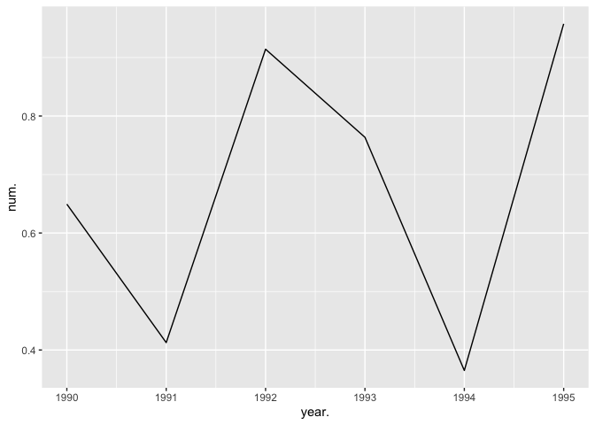
To apply the ggplot grammar of graphics to tb_wide is not problematic due to layers., appropriate care being taken not to mix continuous and discrete variables without further intervention.

library(ggplot2)
library(tibble)
set.seed(137)
yr. <- 1990:1995
nm. <- runif(6)
tx. <- letters[1:6]
fc. <- paste0(tx., round(nm. * 100, 0))
tb_wide <- tibble(year. = yr., num. = nm., txt. = tx., fact. = fc.) # , key = year., index = year.)
tb_wide
#> # A tibble: 6 x 4
#>   year.  num. txt.  fact.
#>   <int> <dbl> <chr> <chr>
#> 1  1990 0.649 a     a65  
#> 2  1991 0.413 b     b41  
#> 3  1992 0.914 c     c91  
#> 4  1993 0.764 d     d76  
#> 5  1994 0.365 e     e36  
#> 6  1995 0.958 f     f96
p <- ggplot(data = tb_wide, aes(x = year.)) + geom_line(aes(y = num.))
p

Created on 2019-11-14 by the reprex package (v0.3.0)

As for tstibble, I don't see why the class changes anything. The underlying problem is the mix of num, txt and fact objects, of which the second and third cannot be property coerced to num.

The approach, when coercion is unavailable would seem to be facet or glob.

As always, I may be wrongheaded, but does this advance the question?

2 Likes

Since you mention the Gospel of Hadley I would like to point out that the tidy data idea is very close to the subject of database normalization, so help me Codd.

This was a hot topic in the seventies and eighties, when disk space was expensive, and technology constraints were felt more acutely than they are now.

3 Likes

This topic was automatically closed 21 days after the last reply. New replies are no longer allowed.