Statistical test for linearity

Hi,

What statistical test measures which of k independent variables are linear with respect to the dependent variable for use in linear regression? I am not looking for an answer involving a graph.

Is the answer any different for linearity with respect to the logit of a binary dependent variable for use in logistic regression?

Thank you.

There are, of course, a very large number of ways that a model can depart from linearity. But a pretty good--and simple--way to test for lots of forms of nonlinearity is to add the variable x^2 to the equation and see if it's significant. (Adding x^2 is the most simple form of putting in a Taylor series expansion.)

Linearity (method comparison) > Method comparison / Agreement > Statistical Reference Guide | Analyse-it® 6.15 documentation

A CUSUM is a measure of the linearity, defined as a running sum of the number of observations above and below the fitted regression line. When the relationship is linear it is expected the points above and below the line are randomly scattered, and the CUSUM statistic is small. Clusters of points on one side of the regression line produce a large CUSUM statistic.

A formal hypothesis test for linearity is based on the largest CUSUM statistic and the Kolmogorov-Smirnov test. The null hypothesis states that the relationship is linear, against the alternative hypothesis that it is not linear. When the test p-value is small, you can reject the null hypothesis and conclude that the relationship is nonlinear.

@nirgrahamuk, could you show how to do this in R? I'm curious to learn something new.

I apologize; Ive not done it myself, I wouldnt have need to...
In my own work I would look at a plot, or just try the linear regression and see what comes of it. I only found this suggestion by a quick google around. I might play with it later and see if I can understand it in more depth myself. I've used Kolmogorov Smirnov before in various ways. but not seen this CUSUM statistic

In ordinary least squares regression, with a response (dependent) variable Y and one or more treatment (independent) variables X, we are fitting an equation that is linear in its parameters

Y = β_0 + β_1X_1 + β_2X_2 \dots + β_nX_n + ε_i

And below, I've spoiled the rest of my answer because it is wrong. What I should have gone on to say is

A model with independent variables that are logarithmic, exponential, squared, cubic, quadratic, or raised to any power can still be linear in the parameters if the model can be represented as a linear combination of the parameters.

So, not only the above model with no variable raised to a power, a quadratic model

Y = β_0 + β_1X_1 + β_2X{_2}^2 \dots + β_nX_n + ε_i

is also linear in the parameters. How could I have gone so wrong? (Many possibilities, I know.) The answer is that I didn't go on to take linear algebra in 1968, the way I should have done. That lame excuse is more than offset by entirely neglecting my training and practice as a lawyer: the same damned word can have different meanings in different contexts.

Here, I was conflating the parameters of a function, such as variables, with the parameters of an equation, such as coefficients, the \beta terms.

Feel free to click through the spoiler cloud to see the underlying BS.

and deciding whether the model has sufficient utility to be satisfactory for the purposes to which it will be put. What if a better model exists that is not linear in its parameters?

Y = β_0 + β_1X_1 + β_2X{_2}^2 \dots + β_nX_n + ε_i

How would we discover what combination of parameters and equations of quadratic, cubic, quartic, quintic and an infinite choice of nth-order polynomials? We can get a feeling for how quickly to expect exploding skulls with

demo(stats::nlm)

But back to sanity. We don't set about modeling data from a standpoint of pure ignorance. We done exploratory data analysis, plotted with pairs() and otherwise gotten an idea that an X variable might not be of linear order. We can check that by Y = β_0 + β_1X_1 + β_2X{_1}^2 + ε_i. If the model is truly linear in X_1, then β_2 will equal 0. When it is not, there are the link function options in glm to adjust.

In the case of Y \in \{0,1\}, the same principle of linearity in the parameters applies. But as it's late here, I'm going to put Harrell's RMS aside.

Here's some sample data that is obviously quadratic, and code to calculate cumsum in linear and quadratic cases. I'm not sure what to do next with K-S.

df <- data.frame(x=c(6, 9, 12, 14, 30, 35, 40, 47, 51, 55, 60),
y=c(14, 28, 50, 70, 89, 94, 90, 75, 59, 44, 27))

linear <- lm(df$y ~ df$x)
summary(linear)
df$fit_linear <- fitted(linear)
df$ab_linear <- ifelse(df$fit_linear >= df$y, 1, -1)
df$csum_linear <- cumsum(df$ab_linear)

plot(df$x, df$y, pch=16, cex = 1.3, col = "blue", main = "Linear")
abline(lm(df$y ~ df$x), col="firebrick1")

quad <- lm(df$y ~ df$x + I(df$x^2))
summary(quad)
df$fit_quad <- fitted(quad)
df$ab_quad <- ifelse(df$fit_quad >= df$y, 1, -1)
df$csum_quad <- cumsum(df$ab_quad)
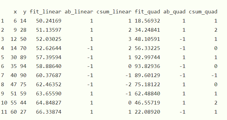
df

bo <- quad$coefficient[1]
b1 <- quad$coefficient[2]
b2 <- quad$coefficient[3]
equation = function(x){bo+b1x+b2x^2}
plot(df$x, df$y, pch=16, cex = 1.3, col = "blue", main = "Quadratic" )
curve(equation, from=0, to=3500, n=10000, add=TRUE, col="firebrick1")

What about this way in order to check it:

https://sscc.wisc.edu/sscc/pubs/RegDiag-R/linearity.html#main

https://cran.r-project.org/web/packages/rempsyc/vignettes/assumptions.html

model <- lm(mpg ~ wt * cyl + gear, data = mtcars)
library(lmtest)

resettest(model)

RESET test

data:  model
RESET = 0.77957, df1 = 2, df2 = 25, p-value = 0.4694

checking with plots:

library(performance)
library(see)

check_model(model)

Note that the reset test essentially adds the square and higher order terms and tests for significance.

Can you please explain in simple, basic, plain English what does it mean ?

Not sure if this will help, but...
A regression that is linear in the variables looks like
y = \beta_1 x + \epsilon

The equation
y = \beta_1 x + \beta_2 x^2 + \epsilon

has a curve in it due to the x^2 term. The idea is to test if \beta_2=0, in which case the curve isn't really there.

Including the term x^2 allows only for a very simple kind of curve. The RESET test can also consider, x^3, x^4 etc., and so can compare the straight line to fancier curves.

Thank you, very helpful.

So is there a better test (than RESET) to test linearity like in OP question.
Almost everything in google revolving around scatter plot and visual, subjective assessment.

Not to my knowledge, but maybe someone else here has a suggestion.

What about ncvTest() ?

https://stats.stackexchange.com/questions/58941/ncvtest-from-r-and-interpretation

This is test for homoscedasticity/heteroscedasticity. If this assumption is not met (homoscedasticity) it will indicate non-linear relationship ?

This is helpful as well:
https://forum.posit.co/t/how-to-check-the-linearity-assumption-in-survey-package/155990/8

homoscedasticity has nothing to do with linearity.
regTermTest is a way to implement the reset test.

OK, I think several of you have answered my question: The procedure is to run a nested F test with a full model containing polynomial terms, versus a reduced model not containing polynomial terms, and see if the full model has significance. Polynomial terms are not the only way for there to be nonlinearity, but a continuous and differentiable function is expressible as a Taylor Series of polynomials, and a square and cube term are probably enough to answer the issue. Is this accurate, and if so thank you to everyone who replied.

2 Likes

You could fit a GAM with penalized splines instead of a linear regression and look for estimated degrees of freedom close to 1 as an indicator of linearity. This approach would allow you to use a binomial distribution with logit-link as well.

Can you @Aariq show how to do it using sample data, this way everybody could benefit from it.

Noam ross has a great course on GAMs online that I'd recommend going through at the very least if it's something you're unfamiliar with: https://noamross.github.io/gams-in-r-course/

Here's an example of fitting a GAM and looking at estimated degrees of freedom (EDF):

library(mgcv)
#> Loading required package: nlme
#> This is mgcv 1.8-42. For overview type 'help("mgcv-package")'.
library(gratia) #for plotting and data_sim()
set.seed(123)
df <- data_sim("eg1", dist = "binary")

m <- gam(y ~ s(x0) + s(x1) + s(x2) + s(x3), family = "binomial", data = df, method = "REML")

draw(m, residuals = TRUE)

summary(m)
#> 
#> Family: binomial 
#> Link function: logit 
#> 
#> Formula:
#> y ~ s(x0) + s(x1) + s(x2) + s(x3)
#> 
#> Parametric coefficients:
#>             Estimate Std. Error z value Pr(>|z|)    
#> (Intercept)    5.775      0.975   5.923 3.16e-09 ***
#> ---
#> Signif. codes:  0 '***' 0.001 '**' 0.01 '*' 0.05 '.' 0.1 ' ' 1
#> 
#> Approximate significance of smooth terms:
#>         edf Ref.df Chi.sq  p-value    
#> s(x0) 3.058  3.803 18.788 0.000821 ***
#> s(x1) 3.581  4.436 34.183 1.64e-06 ***
#> s(x2) 6.257  7.269 55.327  < 2e-16 ***
#> s(x3) 1.000  1.000  1.752 0.185671    
#> ---
#> Signif. codes:  0 '***' 0.001 '**' 0.01 '*' 0.05 '.' 0.1 ' ' 1
#> 
#> R-sq.(adj) =  0.758   Deviance explained = 74.4%
#> -REML = 70.237  Scale est. = 1         n = 400

Created on 2023-07-10 with reprex v2.0.2

You can see that for s(x3) it draws a straight line and EDF =1 (i.e. just a slope). To test whether the straight line fit is best, maybe you could do some bootstrap estimates of EDF and check that confidence intervals include 1? This is just a very rough idea. You'd want to make sure you're specifying the GAM well and do some thinking about how to devise a test for EDF=1 and be sure it means what I think it means.

1 Like

This topic was automatically closed 42 days after the last reply. New replies are no longer allowed.

If you have a query related to it or one of the replies, start a new topic and refer back with a link.