solution to reading .raw images into R?

[rhoutman]

I was really happy to read this post by SDStat:

Reading .RAW images in R

I would like to read .RAW images in R. I can open those images in ImageJ software using following parameters - Image Type: 16-bit Unsigned Width: XXXX pixels Height: XXXX pixels Offset to first image: 0 bytes Number of Images: 1 Gap between Images: 0 bytes unchecked - White is zero checked - Little-endian byte order unchecked - Open all files in folder unchecked - Use virtual stack [image]

because I am struggling with exactly the same problem!

mdsumner claimed he could solve it, but the answer was never shown.
can someone provide the solution to me?

many thanks!

[rhoutman]

or is there a way to contact @mdsumner directly?

[andresrcs]

You already did, by @name mentioning a person on a post, they get an email notification, just be aware of the @name mentioning policy to avoid a misuse of this feature.

FAQ: Should I @name mention other users in my post?

What is @name mentioning? @name mentioning is when you type someone's username with an @ preceding it. Doing this sends a notification to the user. Depending on their settings, it may also send them an email message. For example, with @JacqueHousteauGram in my text, Jacque here will be dynamically notified in community (and via email if he's configured for it). Please don't use this feature excessively In general, it is considered bad form to @name mention someone not otherwise engaged in the conversation. Why should I limit how much I @name mention others? It can be annoying Active people who were being frequently mentioned in topics were first to request that this practice be minimized…

[Timesaver]

You can try using the readRaw() function in hexView package.

library(hexView) 
readRaw(file, width = NULL, offset = 0, nbytes = NULL, machine = "hex", human = "char", size = switch(human, char = 1, int = 4, real = 8), endian = .Platform$endian, signed = TRUE)

Alternatively you can use the readBin() function.

[mdsumner]

@rhoutman put together an example and I'll do it, the key information in the other post is the screen shot of data-type, width, height, offset, gap, no. of images, little-endian etc. but what is missing is an example file.

readBin() does everything needed, you read raw numeric values from bytes in the .raw file, but then push them into a matrix() in the right order. I don't have any .raw files, but this is exactly what so many other raw-binary format files use it's a good skill to learn.

[rhoutman]

thanks for pointing that out.
I realised I forgot to add the @ in my original post.

[rhoutman]

I have tried to work with readRaw() (which I think is related to readBin as you and @Timesaver have suggested, and although it the arguments seemed logical, I couldn't reproduce an image that looked like it was supposed to.
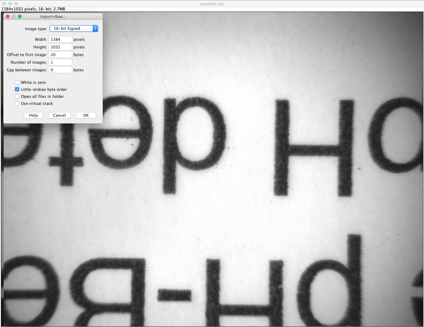
Below is a screenshot of ImageJ settings that do result in the proper image as shown.

The original .raw file can be found here

[mdsumner]

This seems right, there's a lot to unpack (ha ha), I over-read and drop values rather than seek/skip into the file.

16-bit signed means 2-byte integers, offset means we have to skip so many bytes (but I think that is 18 values, not 20). Ironically those 36 bytes probably contain the information we need but you'd need more examples (or the spec.) to know.

  wh <- c(1384, 1032)

## I think the offset is 18, not 20 because
file.info("example.raw")$size/2 - 18
#[1] 1428288
prod(wh)
#> [1] 1428288

v <- readBin("example.raw", what = "integer", 
             n = prod(wh) + 18, size = 2,  
             signed = TRUE, endian = "little")
v <- v[-(1:18)]  ## drop the offset bytes

## check the values
range(v)
#> [1]  233 4095
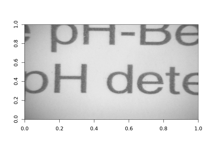
## seems readable in this orientation
image(matrix(v, wh[1], wh[2])[wh[1]:1,], useRaster = TRUE, col = grey.colors(256))

^{Created on 2019-11-27 by the reprex package (v0.3.0)}

HTH

[rhoutman]

yes!
this works beautifully! Thanks so much.
Since you are an expert on the way images 'work' I have another question because sometimes working with images it seems magic happens:
I tried to plot the data as tif file using:

tiff("output.tif", width=wh[1], height=wh[2])
par(c(0,0,0,0))
image(matrix(v, wh[1], wh[2])[wh[1]:1,], useRaster = TRUE, col = grey.colors(256))
dev.off()

and the result is a tiif file with twice the size of the original raw file.
can you explain to me why that is?

[mdsumner]

well, your original data is 16-bit integers so the file is size prod(wh) * 16 + 18. When we plot in R we are assuming a colour model - i.e. we are mapping those raw numeric values to some way of encoding colours - as the ?tiff says

TIFF is a meta-format:
the default format written by ‘tiff’ is lossless and stores RGB
values uncompressed-such files are widely accepted, which is their
main virtue over PNG.

So, potentially for every numeric value we have a 3-bytes to encode RGB (0:255 along 3 axes), so we might expect prod(wh) * 3. Even though we used grey colours, those are expanded (redundantly) into RGB (all the axes have the same value, so greyscale - we have no way of knowing if our encoding is sensible for the data you have, we just stretched out white-to-black along the range of values you have in this particular file - you'd want a different data-value min-max to give absolute colours across all files).

There's some extra bytes for the TIFF format itself:

file.info("output.tif")$size
[1] 4285004
prod(wh) * 3
[1] 4284864

I don't know if tiff() can be used to produce greyscale (a single band), but it can compress so

tiff("output.tif", width=wh[1], height=wh[2], compression = "lzw")
par(c(0,0,0,0))
image(matrix(v, wh[1], wh[2])[wh[1]:1,], useRaster = TRUE, col = grey.colors(256))
dev.off()
file.info("output.tif")$size
[1] 1467824

You would also have some axis cruft around the edges I expect, so use image(, axes = FALSE, xlab = "", ylab = "") to get the cleanest output.

Oh, also beware of useRaster - in this case it probably won't do any interpolation/resampling because you are targetting a device with the dimensions of your matrix (and no margin), but to be safe I'd set useRaster = FALSE, though it will be slower.

I don't know how to render more directly to image files, it's something I wish we could do more easily (magick has some ability here and maybe does what I'm talking about).

[rhoutman]

thanks so much for the clear explanation.
it took me a bit to process and test it al, hence the slow response.
I have something I can work with now.
cheers