Smoother Visualization Techniques for Improved Data Representation

[Shin1]

Hi guys, I'm trying to do a graph for polarity headlines. Is it possible to generate a smoother graph than the current one to represent the data? The current graph appears to be too crowded, and I would like to know if there is a way to make it clearer and easier to interpret

# Criar a lista de 500 datas a partir do dia "2014-02-04"
data_inicial <- as.Date("2014-02-04")
lista_datas <- seq(data_inicial, by = "days", length.out = 500)

# Criar o vetor topic_id com 500 valores 0
topic_id <- rep(0, 500)

# Criar o vetor polaridade com os valores fornecidos
polaridade <- c(-0.45, -0.091666667, 0.016212121, -0.325, 0.060833333, -0.051, -0.018017677, -0.047121212, -0.206666667, 0.03625,
                -0.185, -0.068, -0.079679487, -0.242857143, 0.028541667, -0.028055556, -0.016528926, -0.071666667, -0.35, -0.033095238,
                -0.080740741, -0.124, -0.101666667, -0.26, -0.129375, -0.015454545, -0.136666667, -0.068, -0.257291667, -0.134375,
                -0.103787879, -0.060576923, -0.01375, -0.4125, -0.085, -0.022727273, -0.08715812, -0.013287037, -0.225, -0.034393939,
                -0.103863636, -0.029938272, -0.046212121, -0.172159091, -0.2, -0.196428571, -0.288802083, -0.354166667, -0.325,
                -0.285714286, -0.185, -0.225, -0.172222222, -0.35, -0.291666667, -0.308928571, -0.030606061, -0.325, -0.141388889,
                -0.106818182, -0.01625, -0.0625, -0.211111111, -0.058090278, -0.257291667, -0.054469697, -0.035714286, -0.2625,
                -0.207083333, -0.067575758, -0.001410256, -0.016875, -0.176785714, -0.1565, -0.1045, -0.099230769, -0.048787879,
                -0.197159091, -0.000416667, -0.108888889, -0.061944444, -0.188888889, -0.41875, -0.047619048, -0.145555556, -0.145833333,
                -0.003703704, -0.308333333, -0.109863946, -0.048666667, -0.050771605, -0.071071429, -0.133333333, -0.044074074,
                -0.173981481, -0.031363636, -0.087777778, -0.213333333, -0.135555556, -0.051243386, -0.0434375, -0.188712121,
                -0.3734375, -0.147222222, -0.042245532, -0.030947293, -0.08037037, -0.105357143, -0.085555556, 0.023020833, -0.052,
                -0.119, -0.167777778, -0.3, -0.048611111, -0.246666667, -0.204444444, -0.233333333, -0.116666667, -0.045833333, -0.1,
                -0.135308642, -0.2625, -0.160714286, -0.035982906, -0.017361111, -0.053333333, -0.14, -0.15, -0.079166667, -0.075,
                -0.101428571, -0.35, -0.123097643, 0.013888889, -0.101851852, -0.129166667, -0.191666667, -0.263888889, -0.128935185,
                -0.152777778, -0.133333333, -0.35, -0.218314394, -0.124, -0.1328125, -0.203055556, -0.296875, -0.3625, -0.2625, -0.146666667,
                -0.331944444, -0.10625, -0.115277778, -0.069907407, -0.078311688, -0.142857143, -0.173333333, -0.183333333, -0.011388889,
                -0.126083333, -0.208333333, -0.35, -0.129166667, -0.05952381, -0.114136905, -0.233333333, -0.098809524, -0.165277778,
                -0.062512626, -0.03962963, -0.135185185, -0.2375, 0.07, -0.057638889, -0.081428571, -0.145555556, -0.35, -0.161875,
                -0.0275, 0.025, -0.187962963, -0.35, -0.036071429, -0.100740741, -0.154404762, -0.011458333, -0.223809524, -0.204166667,
                -0.129907407, -0.1621875, -0.195833333, -0.38125, -0.226388889, -0.204861111, -0.122395833, -0.218518519, -0.179166667,
                0.037142857, -0.046296296, -0.069215168, -0.144965278, -0.1375, -0.197013889, -0.151666667, -0.090208333, -0.101851852,
                -0.367857143, -0.175714286, -0.096666667, -0.066481481, -0.083333333, -0.1, -0.09375, -0.133703704, -0.003472222, 0.042708333,
                -0.28, 0.01, 0.0059375, -0.039479167, -0.068320106, -0.116666667, -0.388095238, -0.081666667, -0.180952381, -0.087037037,
                -0.2375, -0.275, -0.054166667, -0.7, -0.233333333, -0.5, 0, 0, -0.075, -0.116666667, -0.023333333, -0.038571429,
                -0.052840909, -0.248015873, -0.104289773, 0.024, -0.014642857, 0.007857143, -0.35, -0.147, -0.064285714, -0.098660714,
                -0.029635642)

# Criar o dataframe combinando as colunas
df <- data.frame(Data = lista_datas, topic_id = topic_id, polaridade = polaridade)

# Visualizar o dataframe
print(df)
 
# Carregar a biblioteca ggplot2
library(ggplot2)

# Criar o gráfico de linha para a polaridade
ggplot(df, aes(x = Data, y = polaridade)) +
  geom_line() +
  labs(title = "Variação da Polaridade ao Longo do Tempo",
       x = "Data",
       y = "Polaridade") +
  theme_minimal() ```

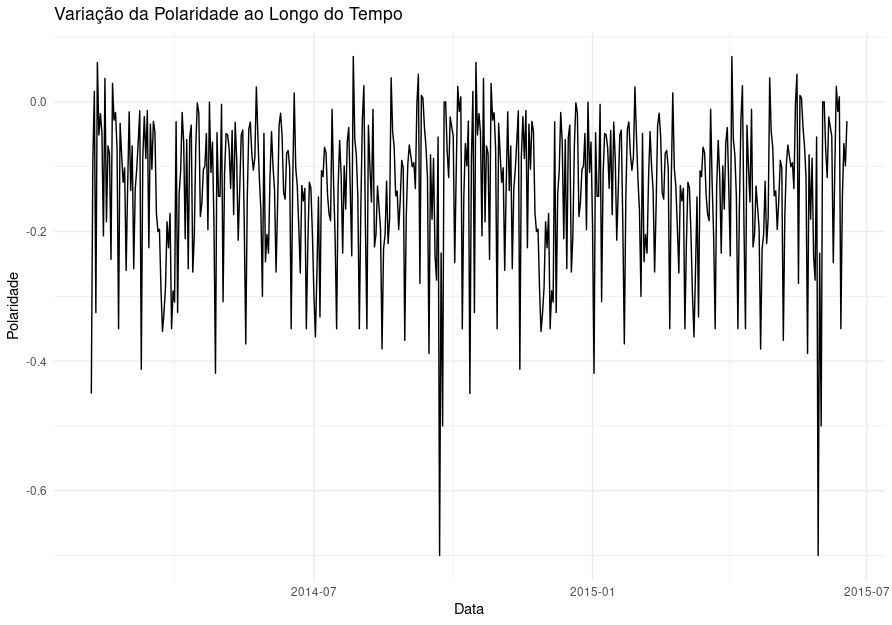
And i would like a graph like this one:

[FJCC]

Your plots did not display correctly in your post, so I'm guessing at what your goal is. You may find geom_smooth() to be useful. Here is code that will plot a smoothed line in addition to your raw data. You can remove the geom_line() if you want to see only the smoothed line and you can tune the span argument to make the line smoother or more like the original data.

ggplot(df, aes(x = Data, y = polaridade)) +
  geom_line() +
  geom_smooth(span = 0.1, se = FALSE) +
  labs(title = "Variação da Polaridade ao Longo do Tempo",
       x = "Data",
       y = "Polaridade") +
  theme_minimal()