Dear all,
can someone help me to add a legend to a SMA regression scatter plot?
Thanks a lot.
I think we need to see your code and some sample data. See
FAQ Asking Questions
A handy way to supply some sample data is the dput() function. In the case of a large dataset something like dput(head(mydata, 100)) should supply the data we need. Just do dput(mydata) where mydata is your data. Copy the output and paste it here between
```
```
This is the output (C_N is SMA regression result).
C_N <- sma (formula = BG ~ NAG_Ure*ID, data = ratios, method = "SMA", multcomp = TRUE, multcompmethod="adjusted", slope.test=1)
dput(C_N)
structure(list(coef = list(A = structure(list(coef(SMA)= c(-16.4783566634032,
2.31667664004903),lower limit= c(-31.5249632736842, 1.19442543034617
),upper limit= c(-1.43175005312227, 4.49336603038784)), class = "data.frame", row.names = c("elevation",
"slope")), B = structure(list(coef(SMA)= c(-16.7172877795454,
2.4150757145656),lower limit= c(-33.4088614103715, 1.17057862100591
),upper limit= c(-0.0257141487193131, 4.98265610051247)), class = "data.frame", row.names = c("elevation",
"slope")), C = structure(list(coef(SMA)= c(-20.6812822359815,
2.86655548963229),lower limit= c(-40.2483805457997, 1.41568434262168
),upper limit= c(-1.11418392616329, 5.80435915532122)), class = "data.frame", row.names = c("elevation",
"slope")), S = structure(list(coef(SMA)= c(10.6634573155724,
-0.86690663793705),lower limit= c(5.31557699404069, -1.82308287806328
),upper limit= c(16.0113376371041, -0.412228718695274)), class = "data.frame", row.names = c("elevation",
"slope"))), nullcoef = list(structure(c(-4.4792232817, 1, NA,
NA, NA, NA), dim = 2:3), structure(c(-4.3330740463, 1, NA, NA,
NA, NA), dim = 2:3), structure(c(-4.0428534861, 1, NA, NA, NA,
NA), dim = 2:3), structure(c(-3.448684813, 1, NA, NA, NA, NA), dim = 2:3)),
commoncoef = list(LR = 6.2870121761651, p = 0.0984514776778647,
b = 2.0475639879336, ci = c(1.40265157613173, 2.95065169198971
), varb = 0.116696344798676, lambda = 4.19251828468254,
bs = structure(c(2.31667664004903, 1.19442543034617,
4.49336603038784, 2.4150757145656, 1.17057862100591,
4.98265610051247, 2.86655548963229, 1.41568434262168,
5.80435915532122, -0.86690663793705, -0.412228718695274,
-1.82308287806328), dim = 3:4, dimnames = list(c("slope",
"lower.CI.lim", "upper.CI.lim"), c("A", "B", "C", "S"
))), df = 3), commonslopetestval = list(LR = 19.111399613096,
p = 0.00074730748838292, b = 1, ci = NA, varb = NA, lambda = 1,
bs = structure(c(2.31667664004903, 1.19442543034617,
4.49336603038784, 2.4150757145656, 1.17057862100591,
4.98265610051247, 2.86655548963229, 1.41568434262168,
5.80435915532122, -0.86690663793705, -0.412228718695274,
-1.82308287806328), dim = 3:4, dimnames = list(c("slope",
"lower.CI.lim", "upper.CI.lim"), c("A", "B", "C", "S"
))), df = 4L), alpha = 0.05, method = "SMA", intercept = TRUE,
call = sma(formula = BG ~ NAG_Ure * ID, data = ratios, method = "SMA",
slope.test = 1, multcomp = TRUE, multcompmethod = "adjusted"),
data = structure(list(BG = c(4.426308275, 4.34966372, 3.865532546,
4.683293513, 4.240838785, 3.78959011, 3.539988617, 3.851137948,
3.81909229, 4.538749784, 5.215412826, 4.208856333, 3.847130421,
6.339150421, 5.317462511, 4.552606853, 3.307303459, 4.385765648,
4.336674511, 4.829372496, 3.416569851, 4.158332878, 5.109054796,
4.706481431, 4.475988564, 3.821945188, 5.437210544, 4.881360655,
3.860798648, 4.317779227, 5.972428997, 4.859032285, 4.561271475,
4.120765413, 4.258429116, 4.627944936, 5.359636377, 4.534059417,
5.507120539, 4.910525401), NAG_Ure = c(7.709524522, 8.478557388,
7.205135904, 6.996607837, 7.114944332, 7.977959573, 7.675999696,
7.355959377, 7.423580005, 7.652775084, 9.249355943, 9.488191629,
8.974777348, 9.595625185, 8.928588088, 8.532474308, 8.569388378,
9.248960291, 9.44244391, 9.102163216, 8.488626332, 9.019256584,
8.937607499, 8.708053122, 9.293168436, 8.733717096, 8.640015504,
8.634049005, 8.440345727, 8.62142294, 9.057427404, 8.534945806,
8.906085485, 8.583331837, 9.008766501, 9.159710848, 8.898366526,
8.977166825, 9.071987451, 8.941960134), ID = structure(c(4L,
4L, 4L, 4L, 4L, 4L, 4L, 4L, 4L, 4L, 1L, 1L, 1L, 1L, 1L, 1L,
1L, 1L, 1L, 1L, 2L, 2L, 2L, 2L, 2L, 2L, 2L, 2L, 2L, 2L, 3L,
3L, 3L, 3L, 3L, 3L, 3L, 3L, 3L, 3L), levels = c("A", "B",
"C", "S"), class = "factor")), terms = BG ~ NAG_Ure * ID, row.names = c(NA,
40L), class = "data.frame"), log = "", variables = c("BG",
"NAG_Ure", "ID"), origvariables = c("BG", "NAG_Ure", "ID"
), formula = BG ~ NAG_Ure * ID, groups = c("A", "B", "C",
"S"), groupvarname = "ID", gt = "slopecom", gtr = "", slopetest = list(
list(F = 9.31827872844995, r = 0.733525955734229, p = 0.0157590234677085,
test.value = 1, b = 2.31667664004903, ci = structure(c(1.19442543034617,
4.49336603038784), dim = 1:2)), list(F = 8.54587929492844,
r = 0.718676511958753, p = 0.0191930406361901, test.value = 1,
b = 2.4150757145656, ci = structure(c(1.17057862100591,
4.98265610051247), dim = 1:2)), list(F = 14.3808204579393,
r = 0.801592842115533, p = 0.00529515380860768, test.value = 1,
b = 2.86655548963229, ci = structure(c(1.41568434262168,
5.80435915532122), dim = 1:2)), list(F = 0.16493541187151,
r = -0.142128305359836, p = 0.695299013550236, test.value = 1,
b = -0.86690663793705, ci = structure(c(-0.412228718695274,
-1.82308287806328), dim = 1:2))), elevtest = list(
list(t = NA_real_, a = -16.4783566634032, p = NA_real_,
a.ci = c(-31.5249632736842, -1.43175005312227), test.value = NA),
list(t = NA_real_, a = -16.7172877795454, p = NA_real_,
a.ci = c(-33.4088614103715, -0.0257141487193131),
test.value = NA), list(t = NA_real_, a = -20.6812822359815,
p = NA_real_, a.ci = c(-40.2483805457997, -1.11418392616329
), test.value = NA), list(t = NA_real_, a = 10.6634573155724,
p = NA_real_, a.ci = c(5.31557699404069, 16.0113376371041
), test.value = NA)), slopetestdone = TRUE, elevtestdone = FALSE,
n = list(A = 10L, B = 10L, C = 10L, S = 10L), r2 = list(A = 0.237345240819926,
B = 0.0629305733849087, C = 0.118431770766887, S = 0.00383926112052757),
pval = list(A = 0.153247511635264, B = 0.484493584148173,
C = 0.330194825995504, S = 0.864977806070641), from = list(
A = 8.5549621626056, B = 8.41268302478244, C = 8.61777223995185,
S = 7.95357464871603), to = list(A = 9.72243320850455,
B = 9.03428854870199, C = 9.17779712797626, S = 6.94744338800689),
groupsummary = structure(list(group = c("A", "B", "C", "S"
), n = c(10L, 10L, 10L, 10L), r2 = c(0.237345240819926, 0.0629305733849087,
0.118431770766887, 0.00383926112052757), pval = c(0.153247511635264,
0.484493584148173, 0.330194825995504, 0.864977806070641),
Slope = c(2.31667664004903, 2.4150757145656, 2.86655548963229,
-0.86690663793705), Slope_lowCI = c(1.19442543034617,
1.17057862100591, 1.41568434262168, -1.82308287806328
), Slope_highCI = c(4.49336603038784, 4.98265610051247,
5.80435915532122, -0.412228718695274), Int = c(-16.4783566634032,
-16.7172877795454, -20.6812822359815, 10.6634573155724
), Int_lowCI = c(-31.5249632736842, -33.4088614103715,
-40.2483805457997, 5.31557699404069), Int_highCI = c(-1.43175005312227,
-0.0257141487193131, -1.11418392616329, 16.0113376371041
), Slope_test = c(1, 1, 1, 1), Slope_test_p = c(0.0157590234677085,
0.0191930406361901, 0.00529515380860768, 0.695299013550236
), Elev_test = c(NA, NA, NA, NA), Elev_test_p = c(NA_real_,
NA_real_, NA_real_, NA_real_)), class = "data.frame", row.names = c(NA,
-4L)), multcompresult = structure(list(ID_1 = c("A", "A",
"A", "B", "B", "C"), ID_2 = c("B", "C", "S", "C", "S", "S"
), Pval = c(0.99999988607908, 0.998152554115843, 0.255256686036767,
0.999595246045009, 0.258183735206681, 0.117986735252858),
TestStat = c(0.00763411962003806, 0.20626683587984, 3.91235318176991,
0.120934448956188, 3.89059875004678, 5.35126054970551
), df = c(1, 1, 1, 1, 1, 1), Slope1 = c(2.31667664004903,
2.31667664004903, 2.31667664004903, 2.4150757145656,
2.4150757145656, 2.86655548963229), Slope2 = c(2.4150757145656,
2.86655548963229, -0.86690663793705, 2.86655548963229,
-0.86690663793705, -0.86690663793705)), row.names = c(NA,
-6L), class = "data.frame"), multcompdone = "slope", multcompmethod = "adjusted"), class = "sma")
Is your dput() output the result of the regression? What we really need is a dput(0)of your raw data. W e also need your complete code. At the moment we do not even know what packages you are using.
Have a look at FAQ Asking Questions
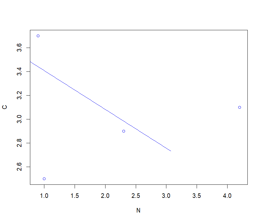
C <- c(2.5,3.1,2.9,3.7)
N <- c(1.0,4.2,2.3,0.9)
C_N <- sma (formula = C ~ N, method = "SMA", slope.test=1)
summary(C_N)
Call: sma(formula = C ~ N, method = "SMA", slope.test = 1)
Fit using Standardized Major Axis
Coefficients:
elevation slope
estimate 3.732528 -0.3250135
lower limit 0.971245 -2.0278976
upper limit 6.493812 -0.0520903
H0 : variables uncorrelated
R-squared : 0.001877934
P-value : 0.95666
H0 : slope not different from 1
Test statistic : r= -0.8092 with 2 degrees of freedom under H0
P-value : 0.19082
plot(C_N)
I'm using smatr(packages).
Is it possibile add a legend to my plot?
Yes but I do not see the need. You only have one variable so a legend is redundant but have a look at Add legends to plots in R software
This function does not accept "SMA objects", so it does not work.
I have simplified the dataset a lot, but it is necessary for me to add a legend.
can you help me?
I do not understand what this means.
For a sibple legend on your plot
library(smatr)
C <- c(2.5,3.1,2.9,3.7)
N <- c(1.0,4.2,2.3,0.9)
C_N <- sma (formula = C ~ N, method = "SMA", slope.test=1)
plot(C_N)
legend(3, 3.6, "points", fill = "blue")
| ID | BG | AP |
|---|---|---|
| A | 5,215412826 | 5,134431419 |
| A | 4,208856333 | 4,424680683 |
| B | 3,416569851 | 4,262466214 |
| B | 4,158332878 | 5,656907089 |
| C | 5,972428997 | 6,088960229 |
| C | 4,859032285 | 5,617862849 |
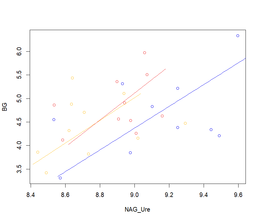
| C_N <- sma (formula = BG ~ NAG_Ure*ID, data = ratios, method = "SMA", multcomp = TRUE, multcompmethod="adjusted", slope.test=1) |
plot(C_N)
legend(3,3.6, "points",legend=c("A", "B","C"), fill = c( "blue", "red", "green"))
legend(3,3.6, "points",legend=c("A", "B","C"), fill = c( "blue", "red", "green"))
The first two numbers are the X, y coordinates on the graph.
Try
legend(8.5 , 6.2, "points",legend=c("A", "B","C"), fill = c( "blue", "red", "green"))
Thanks a lot, now it works.
If I want to add a reference line 1 to 1 like in this image (I.E. Vector model), how could I do?

I'm sorry, I don't understand what text you want to . Can you give me the text that you want to add? That plot is way too "busy".
I would like to add to my sma plot a reference line that passes through axes origin, like dotted line showed in this plot:

Ah, okay I think I see what you want but I am not quite sure how to do it as I, currently, do not see how to extract C & N values from C_N . I'll have to think about it.
Do you want the line going "left bottom" to "right top" like this
xx <- 1:10 ; yy <- 1:10
plot(xx, yy, type = "l")
or "left top" to "right bottom" like this
aa <- 1:10 ; bb <- 10:1
plot(aa, bb, type = "l")
"left bottom" to "right top"
Why if I add a fourth categorical variable (i.e. "A", "B", "C", "D") it doesn't work anymore since it doesn't give the legend anymore?
I do not know. I need to see all your code.
| A | 5,215412826 | 5,134431419 |
|---|---|---|
| A | 4,208856333 | 4,424680683 |
| B | 3,416569851 | 4,262466214 |
| B | 4,158332878 | 5,656907089 |
| C | 5,972428997 | 6,088960229 |
| C | 4,859032285 | 5,617862849 |
| S | 4,426308275 | 3,294318298 |
| S | 4,34966372 | 2,286241941 |
| S | 3,865532546 | 2,530134905 |
| C_N <- sma (formula = BG ~ NAG_Ure*ID, data = ratios, method = "SMA", multcomp = TRUE, multcompmethod="adjusted", slope.test=1) | ||
| plot(C_N) |
legend(8.5 , 6.2, "points",legend=c("A", "B","C"), fill = c( "blue", "red", "green"))