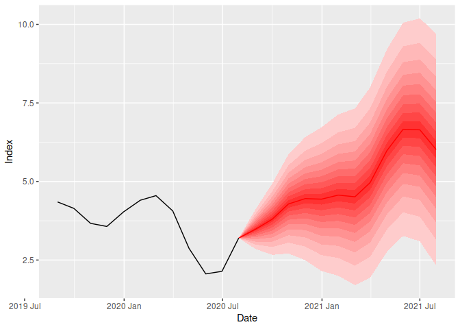
show_gap argument in autoplot function provides error

sablier · September 7, 2020, 2:11am

I am using the fable package to create a fanplot. Everything works fine, however when I try to add the show_gap = F argument in the autoplot function I get the following error

Error: Distributions must have the same `dimnames` to be combined.

Any solutions to solve this?

Here is my dataset

structure(list(Date = c("2003/01/31", "2003/02/28", "2003/03/31", 
"2003/04/30", "2003/05/31", "2003/06/30", "2003/07/31", "2003/08/31", 
"2003/09/30", "2003/10/31", "2003/11/30", "2003/12/31", "2004/01/31", 
"2004/02/29", "2004/03/31", "2004/04/30", "2004/05/31", "2004/06/30", 
"2004/07/31", "2004/08/31", "2004/09/30", "2004/10/31", "2004/11/30", 
"2004/12/31", "2005/01/31", "2005/02/28", "2005/03/31", "2005/04/30", 
"2005/05/31", "2005/06/30", "2005/07/31", "2005/08/31", "2005/09/30", 
"2005/10/31", "2005/11/30", "2005/12/31", "2006/01/31", "2006/02/28", 
"2006/03/31", "2006/04/30", "2006/05/31", "2006/06/30", "2006/07/31", 
"2006/08/31", "2006/09/30", "2006/10/31", "2006/11/30", "2006/12/31", 
"2007/01/31", "2007/02/28", "2007/03/31", "2007/04/30", "2007/05/31", 
"2007/06/30", "2007/07/31", "2007/08/31", "2007/09/30", "2007/10/31", 
"2007/11/30", "2007/12/31", "2008/01/31", "2008/02/29", "2008/03/31", 
"2008/04/30", "2008/05/31", "2008/06/30", "2008/07/31", "2008/08/31", 
"2008/09/30", "2008/10/31", "2008/11/30", "2008/12/31", "2009/01/31", 
"2009/02/28", "2009/03/31", "2009/04/30", "2009/05/31", "2009/06/30", 
"2009/07/31", "2009/08/31", "2009/09/30", "2009/10/31", "2009/11/30", 
"2009/12/31", "2010/01/31", "2010/02/28", "2010/03/31", "2010/04/30", 
"2010/05/31", "2010/06/30", "2010/07/31", "2010/08/31", "2010/09/30", 
"2010/10/31", "2010/11/30", "2010/12/31", "2011/01/31", "2011/02/28", 
"2011/03/31", "2011/04/30", "2011/05/31", "2011/06/30", "2011/07/31", 
"2011/08/31", "2011/09/30", "2011/10/31", "2011/11/30", "2011/12/31", 
"2012/01/31", "2012/02/29", "2012/03/31", "2012/04/30", "2012/05/31", 
"2012/06/30", "2012/07/31", "2012/08/31", "2012/09/30", "2012/10/31", 
"2012/11/30", "2012/12/31", "2013/01/31", "2013/02/28", "2013/03/31", 
"2013/04/30", "2013/05/31", "2013/06/30", "2013/07/31", "2013/08/31", 
"2013/09/30", "2013/10/31", "2013/11/30", "2013/12/31", "2014/01/31", 
"2014/02/28", "2014/03/31", "2014/04/30", "2014/05/31", "2014/06/30", 
"2014/07/31", "2014/08/31", "2014/09/30", "2014/10/31", "2014/11/30", 
"2014/12/31", "2015/01/31", "2015/02/28", "2015/03/31", "2015/04/30", 
"2015/05/31", "2015/06/30", "2015/07/31", "2015/08/31", "2015/09/30", 
"2015/10/31", "2015/11/30", "2015/12/31", "2016/01/31", "2016/02/29", 
"2016/03/31", "2016/04/30", "2016/05/31", "2016/06/30", "2016/07/31", 
"2016/08/31", "2016/09/30", "2016/10/31", "2016/11/30", "2016/12/31", 
"2017/01/31", "2017/02/28", "2017/03/31", "2017/04/30", "2017/05/31", 
"2017/06/30", "2017/07/31", "2017/08/31", "2017/09/30", "2017/10/31", 
"2017/11/30", "2017/12/31", "2018/01/31", "2018/02/28", "2018/03/31", 
"2018/04/30", "2018/05/31", "2018/06/30", "2018/07/31", "2018/08/31", 
"2018/09/30", "2018/10/31", "2018/11/30", "2018/12/31", "2019/01/31", 
"2019/02/28", "2019/03/31", "2019/04/30", "2019/05/31", "2019/06/30", 
"2019/07/31", "2019/08/31", "2019/09/30", "2019/10/31", "2019/11/30", 
"2019/12/31", "2020/01/31", "2020/02/29", "2020/03/31", "2020/04/30", 
"2020/05/31", "2020/06/30", "2020/07/31"), Index = c(12.5394429962958, 
11.0749627219736, 10.6160246946718, 9.01293217207704, 8.48325673013808, 
7.36979166666671, 5.15252499359136, 4.81896991330946, 3.19727031467203, 
0.896525961897554, -1.42734096222467, -1.63450903281305, -1.9992685602829, 
-1.58652672687324, -1.6986168405727, -1.81576080377692, -1.80365573175161, 
-1.54014067426637, -0.841053144807469, -1.25273656044759, -0.551065393093331, 
0.505985437492318, 2.25939333416558, 2.19890054972502, 2.06493344943399, 
1.79811507936507, 1.93779313749691, 2.13290593021827, 1.87376725838251, 
1.57654883606357, 2.12661339889371, 2.50030791969453, 2.56126092845703, 
2.39440078585458, 1.77001953124998, 2.01711491442544, 2.09628275441811, 
2.18053356072598, 1.86463252209708, 1.79864799613714, 2.43223620522757, 
3.39517400266771, 3.34617236398649, 3.88127853881295, 4.05811021731306, 
4.48495023384112, 4.51001559313906, 4.81725584182142, 5.18085233377106, 
4.91177873152131, 5.32509211933925, 5.96466263488684, 6.04843473124634, 
6.02791134044793, 6.20778010715122, 6.15384615384604, 6.48436598592366, 
6.89773901067365, 7.23057500286921, 7.56830913456041, 8.2590626562058, 
8.93455784574468, 9.61518229535587, 9.40444728709116, 9.7873069238408, 
10.5874547275179, 11.2053626634126, 11.1931690929451, 11.2534102724298, 
10.5783475116389, 10.2351202743663, 9.293466475059, 8.47176079734218, 
8.92561983471076, 9.13539967373573, 8.91410048622365, 8.36012861736335, 
7.13153724247226, 6.71875, 6.36645962732918, 6.01851851851853, 
5.69230769230771, 5.69230769230771, 6.16332819722649, 5.81929555895866, 
5.4628224582701, 4.78325859491777, 4.31547619047619, 4.30267062314538, 
3.9940828402367, 3.51390922401171, 3.35766423357664, 3.20232896652111, 
3.34788937409025, 3.49344978165937, 3.33817126269955, 3.61794500723589, 
3.59712230215827, 3.99429386590586, 4.27960057061341, 4.55192034139402, 
5.1209103840683, 5.37482319660536, 5.22598870056497, 5.64174894217206, 
6.19718309859156, 6.18846694796062, 6.32022471910112, 6.28491620111733, 
6.25, 6.03566529492454, 6.29274965800275, 5.71428571428572, 5.54803788903924, 
4.83221476510067, 5.23489932885908, 5.4739652870494, 5.57029177718831, 
5.69536423841059, 5.81241743725229, 5.51905387647833, 5.88235294117647, 
6.08020698576974, 5.7915057915058, 5.53410553410554, 5.51282051282052, 
6.40204865556979, 6.37755102040816, 6.0759493670886, 5.52763819095479, 
5.38847117794485, 5.24344569288391, 5.72851805728518, 5.92592592592591, 
5.97560975609757, 6.20437956204378, 6.82926829268291, 6.80437424058324, 
6.61853188929, 6.47482014388487, 5.96658711217184, 5.95238095238095, 
5.82639714625446, 5.33807829181494, 4.4758539458186, 4.07925407925407, 
4.02761795166859, 4.58190148911799, 4.337899543379, 4.55062571103526, 
4.62753950338601, 4.5045045045045, 4.5045045045045, 4.49438202247192, 
4.7191011235955, 5.18018018018018, 6.20067643742954, 6.94288913773797, 
6.52654867256637, 6.46221248630887, 6.56455142231946, 6.52883569096845, 
6.4724919093851, 6.25, 6.46551724137931, 6.77419354838709, 6.86695278969955, 
7.0663811563169, 6.79405520169851, 6.49214659685864, 6.12668743509865, 
5.24691358024691, 5.33880903490758, 5.00510725229826, 4.35663627152989, 
4.56389452332657, 4.8582995951417, 4.63242698892246, 4.41767068273093, 
4.49999999999999, 4.27435387673958, 3.83480825958702, 3.71819960861057, 
4.3010752688172, 4.28849902534114, 4.37743190661479, 5.04854368932039, 
4.84966052376334, 4.82625482625483, 5.004812319538, 5.09615384615385, 
4.40191387559807, 3.90848427073403, 4.0719696969697, 4.52830188679245, 
4.40487347703842, 4.39252336448599, 4.47343895619758, 3.97412199630314, 
4.34782608695652, 4.14364640883977, 3.66636113657195, 3.56816102470265, 
4.03299725022914, 4.40366972477064, 4.54959053685169, 4.06137184115523, 
2.87253141831239, 2.05908683974934, 2.14094558429974, 3.2)), row.names = c(NA, 
-211L), class = c("tbl_df", "tbl", "data.frame"))

And the code that I've used

library(tidyverse)
library(tsibble)
library(fable)

remove(list = ls())

data <- read_excel(path = 'Data/SACPI.xlsx', col_names = T) 

data <- data %>% mutate(Index = (Index/lag(Index,12) - 1)*100) %>% 
  drop_na()

# Create a tsibble

data <- data %>% 
  mutate(Date = yearmonth(Date)) %>%
  as_tsibble(index=Date)

# Create an Arima model

arima_model <- data %>%
  model(arima = ARIMA(Index))

# Simulate forecasts and plot

fan <- arima_model %>% forecast(h="1 year") 

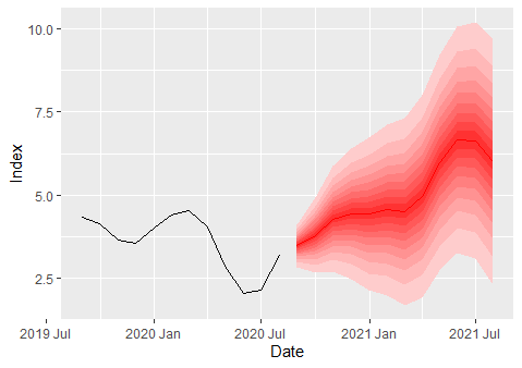
autoplot(fan, data %>% slice(tail(row_number(), 12)), level=seq(10,90,by=10),color = 'red') +
  theme(legend.position="none")

Without the show_gap = F argument, this is how my plot looks like

Rplot05

robjhyndman · September 7, 2020, 7:34am

Your code works for me:

library(tidyverse)
library(tsibble)
library(fable)

# Create a tsibble
data <- data %>%
  mutate(Date = yearmonth(Date)) %>%
  as_tsibble(index = Date)

# Create an Arima model
arima_model <- data %>%
  model(arima = ARIMA(Index))

# Generate forecasts
fc <- arima_model %>% forecast(h="1 year") 

# Plot fan chart
autoplot(
    fc, 
    data %>% slice(tail(row_number(), 12)), 
    level=seq(10,90,by=10),
    color = 'red',
    show_gap = FALSE
  ) +
  theme(legend.position="none")

^{Created on 2020-09-07 by the reprex package (v0.3.0)}

Perhaps try updating the fabletools package from CRAN.

sablier · September 7, 2020, 8:12am

Thanks @robjhyndman, updating my fabletools package managed to work!

sablier · September 7, 2020, 3:59pm

Sorry @robjhyndman if I may ask, there's no way in which I could get this graph into plotly right? I'm assuming that fanplots aren't compatible with ggplotly but just checking in to see whether you have ever managed to get a fanplot into interactive format?

robjhyndman · September 8, 2020, 3:09am

Sorry, no. We may look at this in the future, but nothing on the horizon right now.

technocrat · September 8, 2020, 6:26am

autoplot is a ggplot function and, as such, is amenable to theming to customize displays, with or without plotly.

sablier · September 8, 2020, 10:13pm

Noted @robjhyndman, thanks!

system · September 29, 2020, 10:14pm

This topic was automatically closed 21 days after the last reply. New replies are no longer allowed.

If you have a query related to it or one of the replies, start a new topic and refer back with a link.