setting up bootstrapped test data set to run tune::last_fit

[yonicd]

I am trying to create what is called a visual predictive check (VPC) on the model i tuned using tidymodels. The basic idea would be to create a visual representation of the observed binom confidence interval vs the bootstrapped generated prediction interval based on the tuned model.

To do this I am trying to do

model_split <- initial_split(data, strata = RESPONSE)
model_test <- testing(model_split)
model_boot_test <- rsample::bootstraps(model_test, strata = RESPONSE)

and put that into a last_fit call to create multiple rows of predicted outcomes based on the test data.

last_fit(best_workflow, split = model_boot_test)

this doesnt work because last_fit is expecting an rsplit object and not an rset object

Is there a way to set up the initial data split so i can make this into a model agnostic workflow?

[Max]

last_fit() isn't designed to do that. That function is just a shortcut for this (in pseduocode)

x <- fit(workflow, training_data)
res <- predict(x, testing_data)
metric_set(res)

You'll have to write a small function to do that (or something like that for your application).

Are you trying to get confidence intervals on the test set metrics (via the bootstrap)? If so, I think that you just want:

x <- fit(workflow, training_data)
res <- predict(x, testing_set)
bt <- bootstrap(res) %>% mutate(metric_set_calc)

[yonicd]

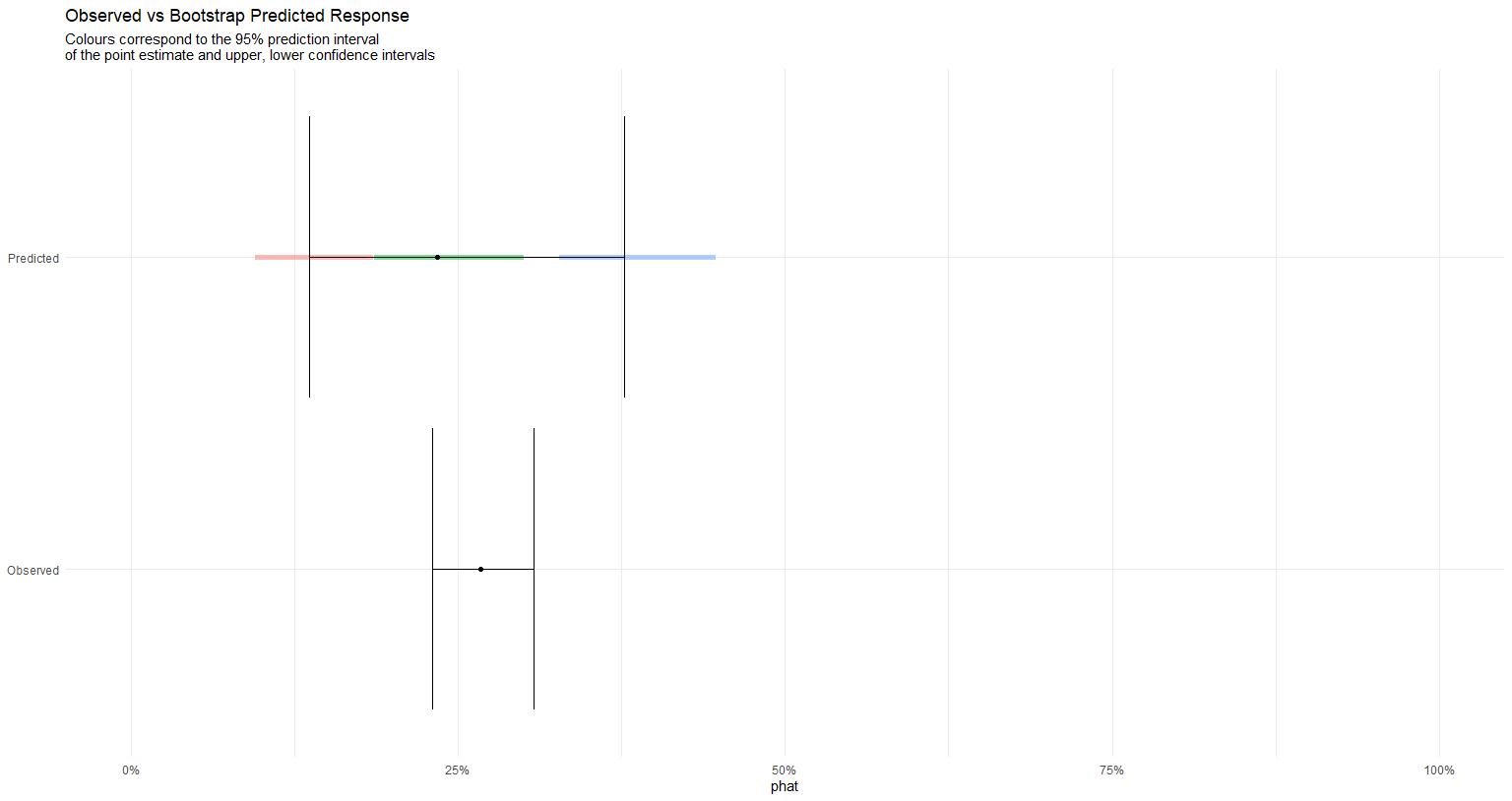
i used this solution in the end. The end result gives the VPC for the predicted response, where the segments represent the 95% prediction intervals for the estimated CI based on the model tuned in the training part.

If there is a simpler way to do that then i'm happy to rework the logic

Targets Pipeline to prep the data

pipe_model_prep <- tar_pipeline(
  tar_target(model_data, 
             pred_setup(subset_hamd,subset_adsl,lb_predict)),
  
  tar_target(model_split, {
    set.seed(3456)
    initial_split(model_data, strata = RESPONSE)
  }),
  
  # Prepare Data
  tar_target(model_train, 
             training(model_split)),
  tar_target(model_cv, 
             rsample::vfold_cv(model_train, strata = RESPONSE)),
  tar_target(model_boot,
             rsample::bootstraps(model_train, strata = RESPONSE)),
  # Prepare Recipe 
  tar_target(model_rec,{
    prepare_recipe(model_train)
  })
)

Targets Pipeline to fit the model

pipe_logistic_model <- tar_pipeline(

  tar_target(logistic_tune, {
    logistic_reg(penalty = tune(),mixture = tune()) %>%
      set_engine('glmnet') 
  }),
  tar_target(logistic_workflow,{
    workflow() %>% 
      add_recipe(model_rec)%>%
      add_model(logistic_tune)
  }),
  tar_target(logistic_fit,{
    set.seed(2020)
    tune_grid(
      logistic_workflow,
      resamples = model_boot,
      grid = dials::grid_regular(dials::penalty(),
                                 dials::mixture(range = c(0.5,1)),
                                 levels = c(50,5)),
      metrics = yardstick::metric_set(yardstick::roc_auc,
                                      yardstick::accuracy)
    )
  }),
  tar_target(logistic_best_workflow,{
    finalize_workflow(
      logistic_workflow,
      logistic_fit%>%select_best(metric = 'roc_auc')
    )
  }),
  tar_target(logistic_last_fit,{
    logistic_best_workflow%>%
      last_fit(split = model_split)
  }),
  tar_target(logistic_best_fit,{
    logistic_best_workflow%>%
      fit(model_train)%>%
      pull_workflow_fit()
  })
  
)

model_test <- testing(model_split)
model_boot_test <- rsample::bootstraps(model_test, strata = RESPONSE)

#create vpc based on best model
vpc_boot <- model_boot_test%>%
  dplyr::mutate(
    test_data = purrr::map(splits,testing),
    pred = purrr::map(test_data,function(object,wf){
      wf%>%
        fit(data = object)%>%
        predict(new_data = object)%>%
        dplyr::mutate(observed = object$RESPONSE)
      
    },wf = logistic_best_workflow)
  )

# calc binomial ci based on Wilson's method 
vpc_boot_unnest <- vpc_boot%>%
  dplyr::mutate(
    pred_ci = purrr::map(pred,function(x){
      binom.confint(x = sum(x$.pred_class=='[3,4,5]'),
                    n = nrow(x),method = 'wilson')%>%
        tibble::as_tibble()
    })
  )%>%
  dplyr::select(id,pred_ci)%>%
  tidyr::unnest(c(pred_ci))

obs_ci <- binom.confint(x = sum(model_data$RESPONSE=='[3,4,5]'),
                        n = nrow(model_data),
                        method = 'wilson')%>%tibble::as_tibble()

dat <- dplyr::bind_rows(
  obs_ci%>%
    dplyr::mutate(id = 'Observed',type = 'Observed'),
  vpc_boot_unnest%>%dplyr::mutate(type = "Predicted")
  )%>%
  dplyr::rename(point = mean)

# melt the data into quantiles
melt_quant <- function(x,probs = c(0.05,0.5,0.95)){
  x%>%
    quantile(probs = probs)%>%
    tibble::as_tibble()%>%
    dplyr::mutate(q = probs)%>%
    list()
}

dat1 <- dat%>%
  dplyr::group_by(type)%>%
  dplyr::summarise(dplyr::across(c(point,lower,upper),list(ci = melt_quant)))%>%
  tidyr::pivot_longer(-type)%>%
  tidyr::unnest(c(value))

pt_dat <- dat1%>%dplyr::filter(q==0.5)%>%tidyr::pivot_wider(names_from = name,values_from=value)

#plot the vpc
ggplot() +
    geom_path(aes(x = value,colour = name,y= type),size = 2,alpha = 0.5,
             data = dat1%>%dplyr::filter(type=='Predicted'&q!=0.5)) + 
    geom_errorbarh(aes(y = type,xmin= lower_ci,xmax = upper_ci),
                data = pt_dat) +
    geom_point(aes(x = point_ci,y = type),data = pt_dat) +
  labs(
    title = 'Observed vs Bootstrap Predicted Response',
    subtitle = 'Colours correspond to the 95% prediction interval\nof the point estimate and upper, lower confidence intervals',
    x = 'phat',y=NULL,colour = 'Predicted') + 
  scale_x_continuous(labels = scales::percent,limits = c(0,1)) + 
  theme_minimal() + 
  theme(legend.position = 'none')

[yonicd]

If i'm not mixing up my use of tidymodels then if i use the model fit for creating simulated predictions i should be taking into account model variation shouldnt i?

the main place i can see that is not right in the code above is

vpc_boot <- model_boot_test%>%
  dplyr::mutate(
    test_data = purrr::map(splits,testing),
    pred = purrr::map(test_data,function(object,wf){
      wf%>%
        fit(data = object)%>%
        predict(new_data = object)%>%
        dplyr::mutate(observed = object$RESPONSE)
      
    },wf = logistic_best_workflow)
  )

which could be changed to the following to make the prediction fully separate from the fit coefficients.

vpc_boot <- model_boot_test%>%
  dplyr::mutate(
    train_data = purrr::map(splits,training),
    test_data = purrr::map(splits,testing),
    pred = purrr::map2(test_data,train_data,function(test,train,wf){
      wf%>%
        fit(data = train)%>%
        predict(new_data = test)%>%
        dplyr::mutate(observed = object$RESPONSE)
      
    },wf = logistic_best_workflow)
  )

(going off of these slides)

[Max]

@yonicd

The end result gives the VPC for the predicted response, where the segments represent the 95% prediction intervals for the estimated CI based on the model tuned in the training part.

I wouldn't call them prediction intervals since they don't account for the model variation. That is proably greater than the test set variation.

Also, not to be nit-picky, but "prediction intervals for the estimated confidence intervals" is not well-defined.