Sequential Modelling in Tidy

[themadprogramer]

I want to model sequential outcomes in tidy, but there is surprisingly little documentation on this. By sequential outcome, I refer to problems where outcomes may depend on previous outcomes: causal graphs, time series, networks...

Background

Let's consider the mtcars dataset. This dataset lists fuel consumption and 10 aspects of automobile design and performance for 32 automobiles from the 1973–74 season. In particular, I'm interested in the relationship between 3 variables: Miles Per Gallon (mpg), Horsepower (hp) and Engine Displacement (dsp).

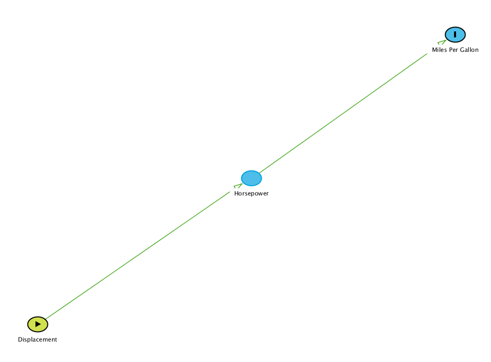
The relationship I assume between these variables is illustrated in the graph above. Here, engine displacement describes the design of an engine: The total volume that is "swept" through the motion of the pistons. The displacement of an engine determines its horsepower, the "power" of an engine. Finally, high horsepower can be costly as it affects the miles per gallon to expect from the vehicle.

With that out of the way, let's see what the mtcars dataset can tell us about this relationship:

library(ggplot2)
library(tidyr)

data(mtcars)

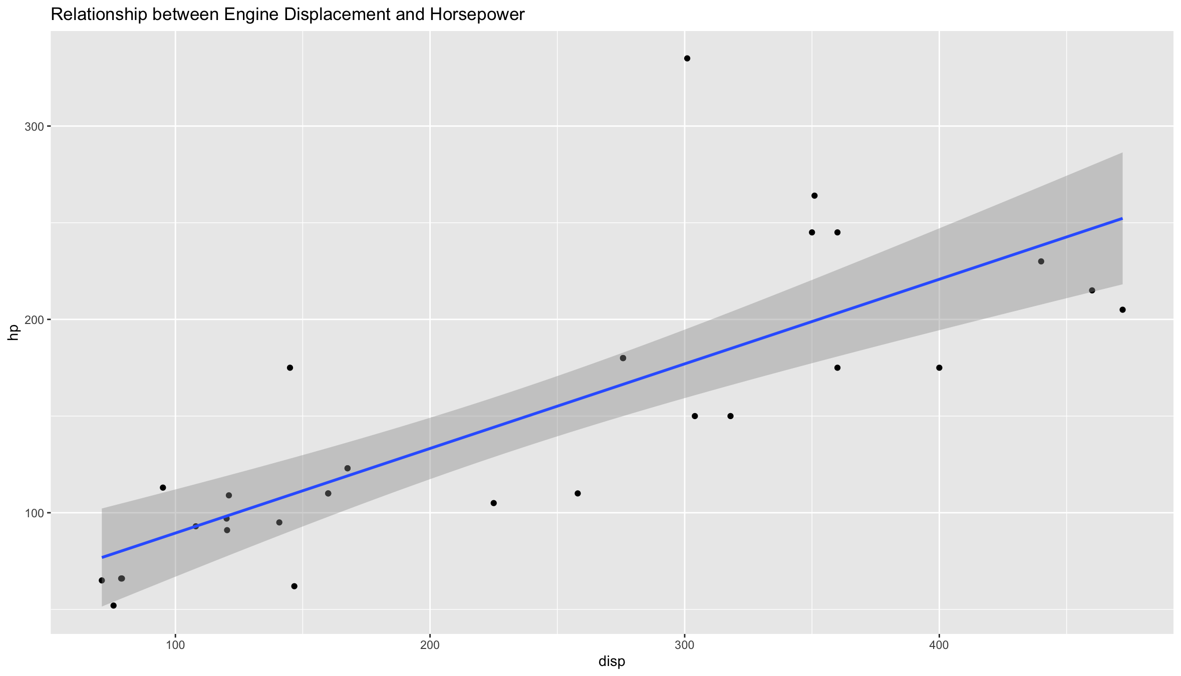
# Modelling a Linear Relationship between hp and dsp
ggplot(mtcars, aes(disp, hp)) +
  geom_point() +
  stat_smooth(method = "lm", size = 1) + 
  ggtitle("Relationship between Engine Displacement and Horsepower")

# Modelling a Quadratic Relationship between mpg and hp
ggplot(mtcars, aes(hp, mpg)) +
  geom_point() +
  stat_smooth(method = "lm", formula = y ~ I(x^2), size = 1) + 
  ggtitle("Relationship between Horsepower and Miles Per Gallon")

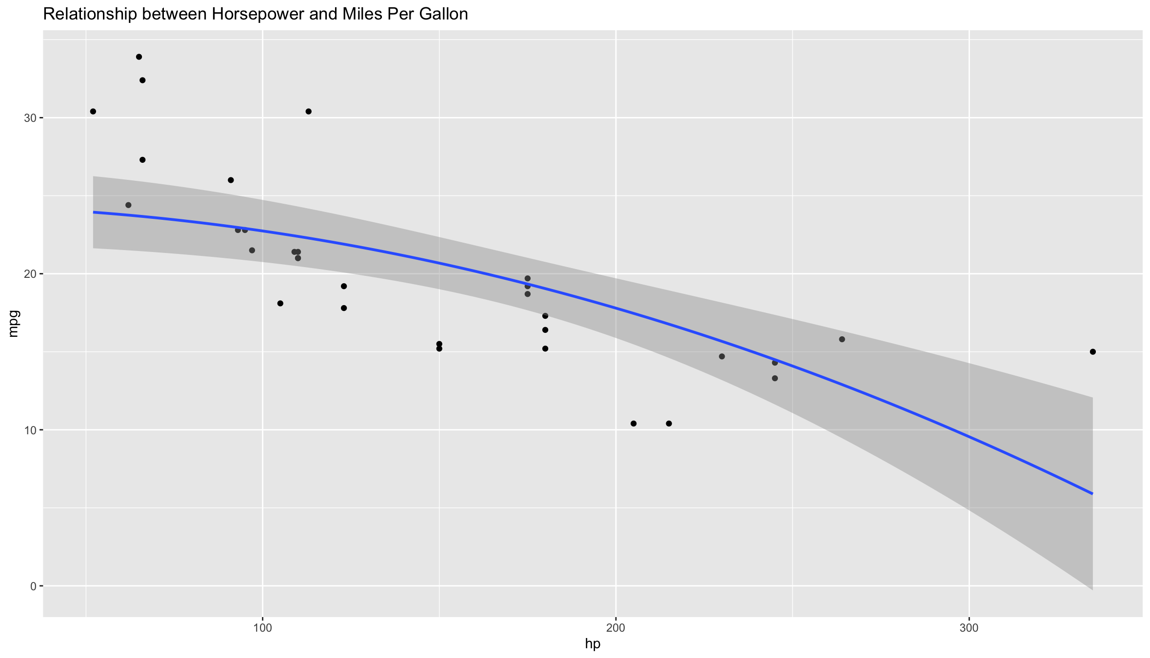
Visually there is a linearly increasing correlation between hp and disp, and a quadratic inverse correlation between mpg and hp.

To represent these separate corelations, I create two parsnip models and fit each.

library(tidyverse)
library(tidymodels)

#Relationship between disp and hp
lm_model_1 <- linear_reg() %>% set_engine('lm') %>% set_mode('regression')
lm_fit_1 <- lm_model_1 %>% fit(hp ~ I(disp^2), data = mtcars)

#Relationship between hp and mpg
lm_model_2 <- linear_reg() %>% set_engine('lm') %>% set_mode('regression')
lm_fit_2 <- lm_model_2 %>% fit(mpg ~ hp , data = mtcars)

lm-fit_1 covers the link between disp and hp; lm-fit_2 covers the link between hp and mpg.

A weakness of tidyverse, or maybe just the way I work with tidy, is that the more chain-relationships there are in a problem the more models I have to create separately. workflows can make this easier, but it is much more geared towards preprocessing.

The Problem

Now let's say I have a new dataset not_mtcars only containing information on engine displacement, and I want to predict both horsepower and miles per galon.

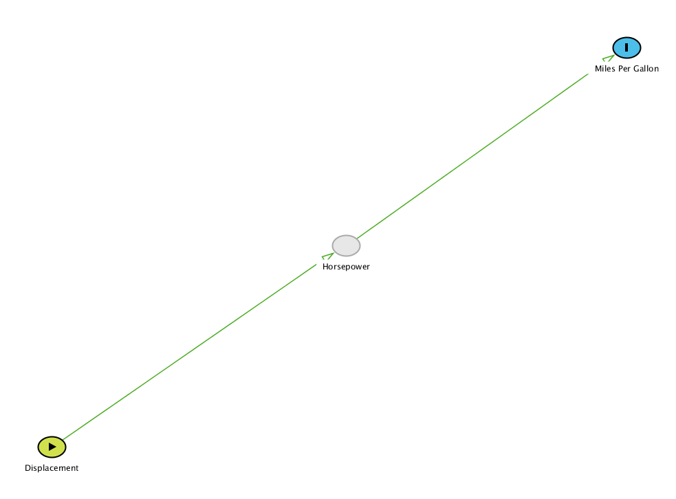
I see that I have two options:

Option A: A Series of Predictors

To get around the dependence here, I first predict hp and add it as a column to the not_mtcars tibble. Then I predict mpg on the updated not_mtcars tibble.

not_mtcars <- tibble(disp=seq(100,501,50)) 

hp_prediction <- predict(lm_fit_1, new_data = not_mtcars)$.pred
not_mtcars <- not_mtcars %>% add_column(hp = hp_prediction)

mpg_prediction <- predict(lm_fit_2, new_data = not_mtcars)$.pred
not_mtcars <- not_mtcars %>% add_column(mpg = mpg_prediction)

head(not_mtcars)

# A tibble: 6 × 3
   disp    hp   mpg
  <dbl> <dbl> <dbl>
1   100  101.  23.2
2   150  111.  22.5
3   200  125.  21.6
4   250  142.  20.4
5   300  164.  18.9
6   350  189.  17.2

Filling-out the table like playing sudoku works. It's fairly easy if we only have a couple of outcomes to consider but doesn't scale super-well for anything more complex (time series).

Option B: Imputation

Another way to handle this is the imputation_step family of functions in recipes. While I think that is a step in the right direction, paying attention to the sequence of imputations and which predictors to impute_with can become overwhelming very quickly.

rec <- recipe(mpg ~ hp+disp, data = mtcars) %>%
  step_impute_linear(
    hp,
    impute_with = imp_vars(disp)
  )  %>% prep(mtcars)
  

sequential_wflow <- 
  workflow() %>% 
  add_model(lm_model_2) %>% 
  add_recipe(rec)

sequential_wflow_fit <- fit(sequential_wflow, data=mtcars)

print(sequential_wflow_fit)

══ Workflow [trained] ═════════════════════════════════════════════════════════════════════════════════════════════════════════════════════════════════════
Preprocessor: Recipe
Model: linear_reg()

── Preprocessor ───────────────────────────────────────────────────────────────────────────────────────────────────────────────────────────────────────────
1 Recipe Step

• step_impute_linear()

── Model ──────────────────────────────────────────────────────────────────────────────────────────────────────────────────────────────────────────────────

Call:
stats::lm(formula = ..y ~ ., data = data)

Coefficients:
(Intercept)           hp         disp  
   30.73590     -0.02484     -0.03035  

Notice also how the linear model generated in this way will also consider disp (normally one step behind) when fitting the mpg.

The Question, for you!

Are these just the "correct" ways to model sequential outcomes in tidy or am I missing something?