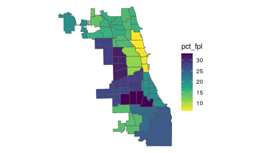
Hello,
I've got PUMs microdata using the tidycensus package. I'm trying to scale these estimates down to a smaller geography using this tutorial.
Below is as sparse as I can make this code, it should all be reproducible (if you have a census API key)
library(magrittr)
library(tidycensus)
library(tigris)
library(sf)
library(ggplot2)
options(tigris_class = "sf")
options(tigris_use_cache = TRUE)

if(Sys.info()['user'] == 'bradyf'){
  census_api_key("MYAPIKEY")
}

# zip map code ----
# read in neighborhood and county map data
chi.link <- "https://data.cityofchicago.org/resource/igwz-8jzy.geojson"
chi      <- read_sf( chi.link ) %>% st_transform( 4326 ) %>%
  mutate(area_ft_cca = as.numeric(st_area(.))))
#ggplot(chi) + geom_sf() +   geom_sf_text(aes(label = community),size=2)
# get PUMs income data ----
pums <- get_pums( variables = c('PUMA', 'HINCP', 'ADJINC', 'NP'),
                  state = 'IL',
                  survey = 'acs5',
                  year = 2019 )
# https://www.census.gov/geographies/reference-maps/2010/geo/2010-pumas/illinois.html
# chicago pums
chi.pumas <- c( '03420', '03422', '03501', '03502', '03503',
                '03504', '03520', '03521', '03522', '03523',
                '03524', '03525', '03526', '03527', '03528',
                '03529', '03530', '03531', '03532' )
# length(chi.pumas)
# filter to pumas in chicago
pums %<>% filter( PUMA %in% chi.pumas )
pums %<>% distinct( PUMA, SERIALNO, WGTP, NP, HINCP, ADJINC )
# pums %>% distinct(SERIALNO) %>% nrow()
# create fpl threshold for each household in the sample
pums %<>%
  mutate( hhld_inc = as.numeric(HINCP)*as.numeric(ADJINC) ) %>%
  filter( hhld_inc > 0 ) %>%
  mutate( fpl = case_when( NP == 1 ~ 12490,
                           NP == 2 ~ 16910,
                           NP == 3 ~ 21330,
                           NP == 4 ~ 25750,
                           NP == 5 ~ 30170,
                           NP == 6 ~ 34590,
                           NP == 7 ~ 39010,
                           T ~ 43430),
          n = sum(WGTP) )
# total N makes sense (~1m households in chicago)

# calculate n_pop and n_fpl estimates for PUMA ----
pums <- pums %>%
  # in each puma
  group_by(PUMA) %>%
  # indicator for PUMA hhld in FPL band
  mutate(fpl_100_200 = ifelse(hhld_inc > fpl & hhld_inc < fpl * 2, 1, 0)) %>%
  # create PUMA Pop and PUMA FPL
  mutate( puma_pop = sum(WGTP) ,
          puma_fpl_100_200 = WGTP*fpl_100_200) %>%
  summarise(puma_pop = max(puma_pop),
            puma_fpl_100_200 = sum(puma_fpl_100_200))

# bring in pums map ----
il_puma <- pumas(state = "IL", cb = TRUE) %>% st_transform( 4326 )
# ggplot(il_puma) + geom_sf() + theme_void()
# restrict to chicago pumas
chi_puma <- il_puma %>% filter( PUMACE10 %in% chi.pumas )
# ggplot(chi_puma) + geom_sf() + theme_void()
# add area to chicago
chi_puma <- chi_puma %>%
  mutate(area_ft_puma = as.numeric(st_area(.))) %>%
  select(PUMA = PUMACE10, GEOID10, NAME10, area_ft_puma, geometry)
chi_puma_fpl <- chi_puma %>%
  left_join(pums, "PUMA")

# intersect the CCA shapefile with the puma shapefile
cca_level <- st_intersection(x = chi_puma_fpl, chi) %>%
  # take the intersecting area (between puma and CCA)
  mutate(area_ft_intersect = as.numeric(st_area(.)),
         # take the puma pop estimate multiply by
         # area of the intersect (puma/CCA)
         # scaled by the area of the puma
         cca_pop = puma_pop * (as.numeric(st_area(.)) / area_ft_puma),
         # same method for FPL est
         cca_est_fpl_100_200 = puma_fpl_100_200 * (as.numeric(st_area(.)) / area_ft_puma))

# use these population estimates to create a pct of fpl 100-200
cca_fpl <- cca_level %>%
  group_by(community) %>%
  summarize(
    neighdist = first(community),
    n_cca = sum(cca_pop),
    n_fpl = sum(cca_est_fpl_100_200),
    pct_fpl = round(sum(cca_est_fpl_100_200) / sum(cca_pop) * 100, 1))

cca_fpl %>% ggplot() +
  geom_sf(aes(fill = pct_pov), size = .25) +
  scale_fill_viridis_c(direction = -1) +
  theme_void()
My resulting map looks essentially like I'm just applying the PUMA FPL estimate to each CCA, when what I want is to scale the numerator (pop at FPL) and denominator (CCA Pop) by the area of the PUMA that each CCA occupies.

this is a little involved but I figured this was a more appropriate place to post than SO, because it's a tidycensus and estimation problem.
Thanks!
Francisco