I'm new to time series modeling (working through the Hyndman/ Athanasopoulos book) and trying to understand how to represent a non-continuous dataset in R.
I have a dataset of daily absentee ballot returns in an American election. The data is only relevant for about 50 days before the election date, which is always on a Tuesday.
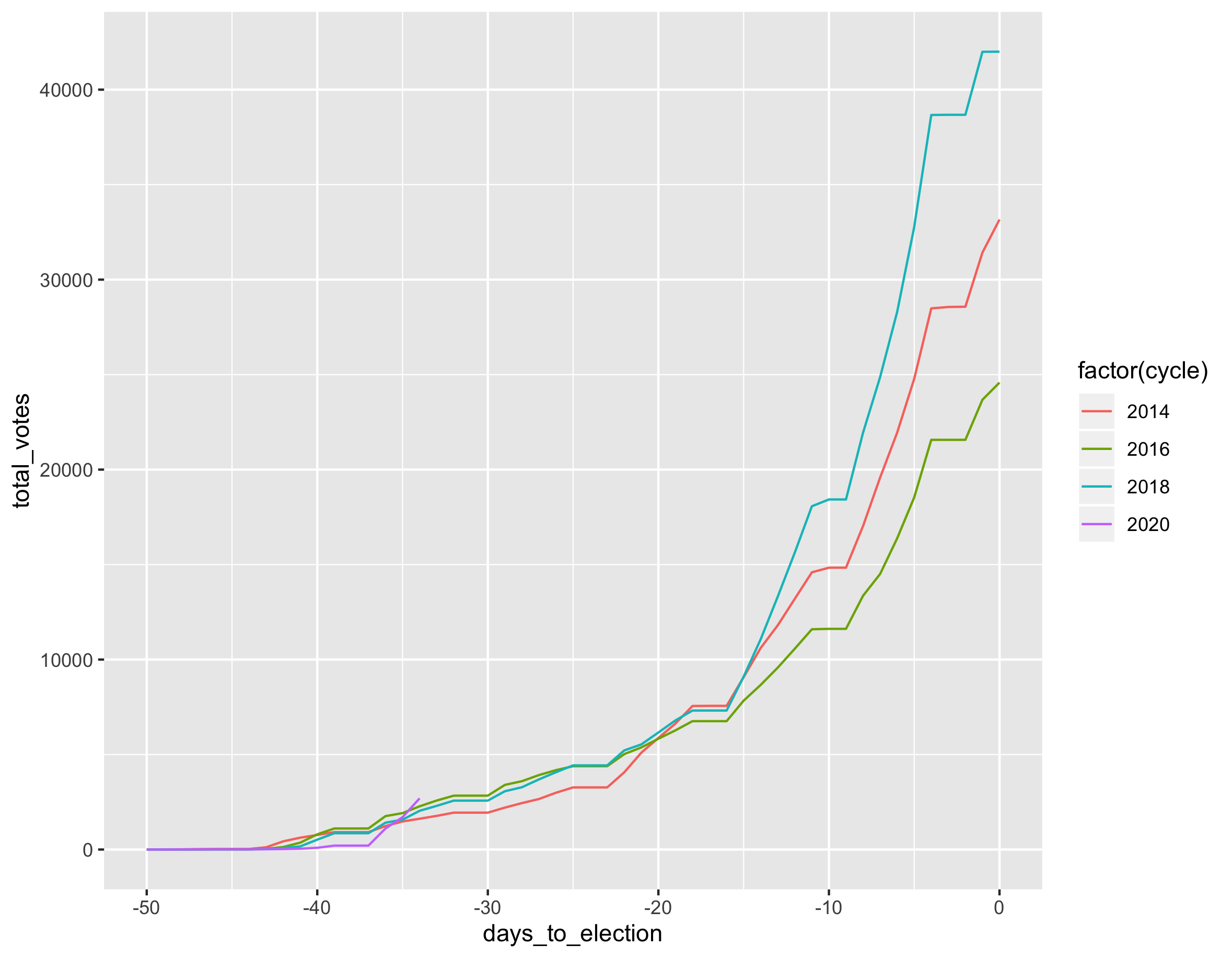
There are four "cycles" of data, each representing a year: 2014, 2016, 2018, and 2020. For each year, there are 51 continuous days' worth of data, indexed starting at -50 (50 days before election day) and ending at 0 (election day).
There is a natural 7-day frequency since some geographies do not count ballots on weekends.
The cumulative number of votes looks like this:
votes <- read.csv('votes.csv')
ggplot(votes,
       aes(x=days_to_election, y=total_votes, color=factor(cycle))) +
  geom_line()
My goal is to explore trends and potentially forecast votes for 2020 based on the previous 4 cycles, but I'm not sure how to represent this dataset since it's not continuous across cycles. Does it make sense to represent this as a single dataset with a frequency of 51 (51 days, including day 0), like this?
vote.ts <- ts(votes$total_votes, start=-50, frequency=51)
ggseasonplot(vote.ts)
My only hesitation is that day "0" of a previous cycle has no relationship to day "-50" of the next cycle and I'm wondering if there's a better way to represent the natural 7-day frequency inherent in the data as well when trying to forecast daily returns (not cumulative).
In other words, there are nested frequencies of "51" (number of days in a cycle) and "7" (days of the week). Or is there a better way to approach this dataset, without thinking of a 51-day cycle as the frequency?