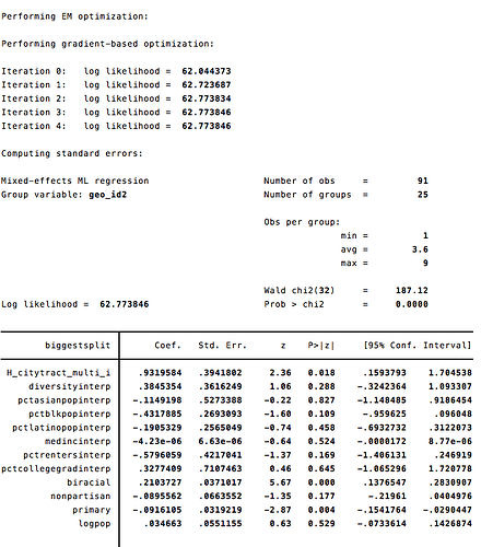
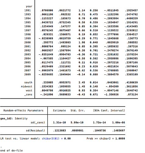
Hi all. I am trying to replicate a Stata paper in R and am having an issue where the results of a multi-level mixed-effects linear regression are very similar, but slightly off (especially the standard errors). I am wondering if anyone knows why this is happening. I am using the exact same dataset in both specifications (which can be found here). The Stata code I am trying to replicate is:
use "/Users/mariaburzillo/Desktop/GOV1006/final_project/racial_polarization_winners.dta", clear

xtmixed biggestsplit H_citytract_multi_i diversityinterp pctasianpopinterp pctblkpopinterp pctlatinopopinterp medincinterp pctrentersinterp pctcollegegradinterp biracial nonpartisan primary logpop  i. year south midwest west if winner==1||geo_id2:
Which gives the following output:
The reprex for my attempt to replicate this in R is:
library(haven)
library(tidyverse)
library(lme4)
#> Loading required package: Matrix
#>
#> Attaching package: 'Matrix'
#> The following objects are masked from 'package:tidyr':
#>
#>     expand, pack, unpack
library(reprex)

# load data

rp <- read_dta("/Users/mariaburzillo/Desktop/GOV1006/final_project/racial_polarization_winners.dta")


# create factor variable for year

rp$year.f <- as.factor(rp$year)

# apply condition that winner == 1 as in Stata regression

rp_sub <- rp %>%
  filter(winner == 1)

# multi-level mixed effects regression with random effects for geo_id2

m1 <- lmer(biggestsplit ~ H_citytract_multi_i + diversityinterp + pctasianpopinterp + pctblkpopinterp + pctlatinopopinterp + medincinterp + pctrentersinterp +  pctcollegegradinterp + biracial + nonpartisan + primary + logpop + year.f + south + midwest + west + (1 | geo_id2), data = rp_sub)
#> Warning: Some predictor variables are on very different scales: consider
#> rescaling
#> boundary (singular) fit: see ?isSingular

# summarize

summary(m1)
#> Linear mixed model fit by REML ['lmerMod']
#> Formula:
#> biggestsplit ~ H_citytract_multi_i + diversityinterp + pctasianpopinterp +
#>     pctblkpopinterp + pctlatinopopinterp + medincinterp + pctrentersinterp +
#>     pctcollegegradinterp + biracial + nonpartisan + primary +
#>     logpop + year.f + south + midwest + west + (1 | geo_id2)
#>    Data: rp_sub
#>
#> REML criterion at convergence: -5.2
#>
#> Scaled residuals:
#>     Min      1Q  Median      3Q     Max
#> -2.0918 -0.4281  0.0000  0.5283  1.9850
#>
#> Random effects:
#>  Groups   Name        Variance Std.Dev.
#>  geo_id2  (Intercept) 0.00000  0.000
#>  Residual             0.02312  0.152
#> Number of obs: 91, groups:  geo_id2, 25
#>
#> Fixed effects:
#>                        Estimate Std. Error t value
#> (Intercept)          -2.419e-01  7.126e-01  -0.339
#> H_citytract_multi_i   9.320e-01  4.937e-01   1.888
#> diversityinterp       3.845e-01  4.530e-01   0.849
#> pctasianpopinterp    -1.149e-01  6.605e-01  -0.174
#> pctblkpopinterp      -4.318e-01  3.373e-01  -1.280
#> pctlatinopopinterp   -1.905e-01  3.213e-01  -0.593
#> medincinterp         -4.225e-06  8.304e-06  -0.509
#> pctrentersinterp     -5.796e-01  5.282e-01  -1.097
#> pctcollegegradinterp  3.277e-01  8.903e-01   0.368
#> biracial              2.104e-01  4.647e-02   4.527
#> nonpartisan          -8.956e-02  8.312e-02  -1.077
#> primary              -9.161e-02  3.998e-02  -2.291
#> logpop                3.466e-02  6.904e-02   0.502
#> year.f1991            7.068e-02  7.788e-02   0.908
#> year.f1993            6.612e-02  1.159e-01   0.570
#> year.f1994            1.153e-01  2.075e-01   0.556
#> year.f1995            4.397e-02  9.424e-02   0.467
#> year.f1996            1.255e-01  1.846e-01   0.680
#> year.f1997            5.762e-02  1.097e-01   0.526
#> year.f1998            2.933e-02  1.963e-01   0.149
#> year.f1999           -2.390e-02  1.027e-01  -0.233
#> year.f2000            2.958e-01  1.871e-01   1.581
#> year.f2001            8.088e-02  1.192e-01   0.679
#> year.f2002            6.029e-02  1.964e-01   0.307
#> year.f2003           -3.516e-02  1.233e-01  -0.285
#> year.f2004           -6.759e-02  1.459e-01  -0.463
#> year.f2005            1.175e-02  1.399e-01   0.084
#> year.f2006            5.294e-02  2.908e-01   0.182
#> year.f2007           -9.040e-02  1.831e-01  -0.494
#> year.f2009           -2.597e-02  2.317e-01  -0.112
#> south                 2.331e-01  1.194e-01   1.953
#> midwest               1.534e-01  1.328e-01   1.156
#> west                  8.498e-02  1.148e-01   0.740
#>
#> Correlation matrix not shown by default, as p = 33 > 12.
#> Use print(x, correlation=TRUE)  or
#>     vcov(x)        if you need it
#> fit warnings:
#> Some predictor variables are on very different scales: consider rescaling
#> convergence code: 0
#> boundary (singular) fit: see ?isSingular
In response to a request for an example from a built-in dataset, etc., here is an alternative reprex using the EmplUK dataset from the plm package:
library(tidyverse)
library(lme4)
#> Loading required package: Matrix
#>
#> Attaching package: 'Matrix'
#> The following objects are masked from 'package:tidyr':
#>
#>     expand, pack, unpack
library(reprex)
library(plm)
#>
#> Attaching package: 'plm'
#> The following objects are masked from 'package:dplyr':
#>
#>     between, lag, lead

# load data from plm package

data("EmplUK", package="plm")

# multi-level mixed effects regression with random effects for firm


m4 <- lmer(wage ~ as.factor(year) + sector + emp + capital +
             output + (1 | firm), data = EmplUK)

# summarize

summary(m4)
#> Linear mixed model fit by REML ['lmerMod']
#> Formula: wage ~ as.factor(year) + sector + emp + capital + output + (1 |
#>     firm)
#>    Data: EmplUK
#>
#> REML criterion at convergence: 4841.1
#>
#> Scaled residuals:
#>     Min      1Q  Median      3Q     Max
#> -6.5171 -0.5067 -0.0280  0.4502  7.9279
#>
#> Random effects:
#>  Groups   Name        Variance Std.Dev.
#>  firm     (Intercept) 21.489   4.636
#>  Residual              3.793   1.948
#> Number of obs: 1031, groups:  firm, 140
#>
#> Fixed effects:
#>                     Estimate Std. Error t value
#> (Intercept)         26.57338    1.55552  17.083
#> as.factor(year)1977 -1.99478    0.27950  -7.137
#> as.factor(year)1978 -2.63032    0.27979  -9.401
#> as.factor(year)1979 -2.51523    0.27983  -8.988
#> as.factor(year)1980 -2.33948    0.28846  -8.110
#> as.factor(year)1981 -1.37792    0.32335  -4.261
#> as.factor(year)1982 -0.33180    0.33480  -0.991
#> as.factor(year)1983  0.49106    0.37275   1.317
#> as.factor(year)1984  0.33148    0.43801   0.757
#> sector              -0.78632    0.14900  -5.277
#> emp                 -0.09098    0.02393  -3.801
#> capital              0.17433    0.05542   3.145
#> output               0.03097    0.01132   2.736
#>
#> Correlation matrix not shown by default, as p = 13 > 12.
#> Use print(x, correlation=TRUE)  or
#>     vcov(x)        if you need it


# write to csv for use in stata

write.csv(EmplUK, file = "empUK.csv" )
The corresponding stata command would be:
xtmixed wage i.year sector emp capital output || firm:
With this example, the outputs are again similar, but they are slightly off. I am trying to see if I can exactly reproduce the Stata code in R.
Thank you for the help! Happy to answer any more questions.

