Replicate graph Rstudio

[RifiFi]

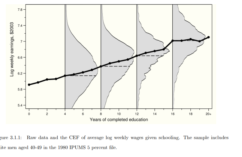
I would like to replicate the figure below but I do not manage to show the Conditional expectation functions for years 4 8 12 16 as below, does anybody have any idea of how to do this ?

Please find below a small reproducible example from
download.file('http://economics.mit.edu/files/397', 'asciiqob.zip')
pums <- read.table("asciiqob.txt", quote=""", comment.char="")
names(pums) <- c('lwklywge', 'educ', 'yob', 'qob', 'pob')

library(ggplot2)
library(data.table)

pums <- data.frame(
  lwklywge = c(5.790019, 5.952494, 5.315949, 5.595926, 6.068915, 5.793871, 6.389161, 6.047781, 5.354861, 5.259597, 5.239404, 5.874553, 6.001272, 5.508173, 5.866414, 5.729413, 5.729413, 5.809437, 6.657937, 6.289252, 6.631926, 6.092223, 5.971912, 5.847161, 6.239488, 6.357876, 6.752745, 6.047781, 6.152528, 4.931287, 3.883974, 6.023867, 5.441835, 6.332576, 4.606131, 6.542389, 4.502584, 5.874553, 4.929898, 5.455957, 6.001272, 6.092223, 5.499443, 6.620201, 6.357876, 6.047781, 5.464891, 6.620201, 5.760175, 5.441835, 5.036578, 6.288895, 5.790019, 5.165335, 6.175587, 5.522294, 5.721887, 6.465816, 5.809455, 3.484194, 6.351859, 6.397207, 4.972081, 5.32084, 5.075799, 5.901214, 6.105608, 5.664895, 7.19918, 5.116621, 6.413932, 5.595926, 6.252534, 5.790019, 3.91452, 5.658208, 6.075346, 5.996763, 5.47783, 5.901214, 6.2148, 5.521961, 6.514023, 5.441835, 6.175587, 6.163517, 5.847161, 5.336521, 6.677495, 5.298817, 6.037274, 6.151647, 5.879942, 6.134774, 5.729413, 5.729413, 6.05978, 5.729413, 5.94949, 5.501258, 4.193435, 6.252904, 6.39066, 6.40316, 5.729413, 5.574272, 5.511972, 6.106466, 5.657489, 6.25563, 5.20833, 5.015112, 5.524257, 5.259597, 5.790019, 5.940434, 5.933976, 6.512002, 6.36195, 5.289349, 7.050939, 6.07424, 6.357876, 6.132656, 6.029436, 5.911682, 6.512002, 5.018934, 6.075096, 5.987852, 5.521845, 5.952494, 6.665316, 5.901214, 6.142306, 5.952494, 6.092223, 6.468604, 6.502446, 6.014215, 5.376904, 5.176258, 5.915003, 5.678696, 5.901214, 5.805772),
  edu = c(12, 11, 12, 12, 12, 11, 11, 12, 11, 7, 10, 12, 14, 12, 16, 12, 16, 8, 16, 9, 16, 11, 3, 10, 12, 12, 18, 10, 11, 13, 12, 12, 12, 10, 6, 13, 8, 16, 12, 12, 12, 17, 12, 6, 12, 12, 12, 12, 12, 12, 5, 12, 9, 8, 11, 8, 14, 8, 11, 11, 12, 8, 12, 8, 7, 12, 17, 12, 20, 6, 13, 8, 12, 12, 6, 4, 12, 8, 12, 12, 13, 9, 12, 19, 12, 12, 13, 12, 16, 15, 12, 12, 12, 8, 10, 13, 8, 11, 12, 4, 6, 12, 18, 8, 17, 8, 8, 12, 7, 13, 14, 12, 12, 8, 7, 12, 12, 12, 8, 9, 12, 9, 12, 18, 8, 8, 12, 12, 10, 14, 12, 2, 16, 12, 17, 16, 14, 18, 12, 16, 12, 12, 9, 16, 11, 12))

reg.model <- lm(lwklywge ~ educ, data = pums)

pums.data.table <- data.table(pums)
educ.means      <- pums.data.table[ , list(mean = mean(lwklywge)), by = educ]
educ.means$yhat <- predict(reg.model, educ.means)

p <- ggplot(data = educ.means, aes(x = educ)) +
  geom_point(aes(y = mean))                +
  geom_line(aes(y = mean))                 +
  ylab("Log weekly earnings, $2003")       +
  xlab("Years of completed education")

[nirgrahamuk]

There's something not right about that zip...

To help us help you, could you please prepare a reproducible example (reprex) illustrating your issue? Please have a look at this guide, to see how to create one:

FAQ: How to do a minimal reproducible example ( reprex ) for beginners

A minimal reproducible example consists of the following items: A minimal dataset, necessary to reproduce the issue The minimal runnable code necessary to reproduce the issue, which can be run on the given dataset, and including the necessary information on the used packages. Let's quickly go over each one of these with examples: Minimal Dataset (Sample Data) You need to provide a data frame that is small enough to be (reasonably) pasted on a post, but big enough to reproduce your issue. Let's say, as an example, that you are working with the iris data frame head(iris) #> Sepal.Length Sepal.Width Petal.Length Petal.Width Species #> 1 5.1 3.5 1.4 0.…

---

Short Version

You can share your data in a forum friendly way by passing the data to share to the dput() function.
If your data is too large you can use standard methods to reduce it before sending to dput().
When you come to share the dput() text that represents your data, please be sure to format your post with triple backticks on the line before your code begins to format it appropriately.

```
( example_df <- structure(list(Sepal.Length = c(5.1, 4.9, 4.7, 4.6, 5, 5.4, 4.6, 
5, 4.4, 4.9), Sepal.Width = c(3.5, 3, 3.2, 3.1, 3.6, 3.9, 3.4, 
3.4, 2.9, 3.1), Petal.Length = c(1.4, 1.4, 1.3, 1.5, 1.4, 1.7, 
1.4, 1.5, 1.4, 1.5), Petal.Width = c(0.2, 0.2, 0.2, 0.2, 0.2, 
0.4, 0.3, 0.2, 0.2, 0.1), Species = structure(c(1L, 1L, 1L, 1L, 
1L, 1L, 1L, 1L, 1L, 1L), .Label = c("setosa", "versicolor", "virginica"
), class = "factor")), row.names = c(NA, -10L), class = c("tbl_df", 
"tbl", "data.frame")))
```

[RifiFi]

@nirgrahamuk Thanks for the advice ! is it better now ? It is basically the first rows of my database

[nirgrahamuk]

I think next step might be to use a parameter 'confidence' to get upper and lower bounds anlong with prediction for the lm prediction, however these provide 3 columns of info rather than 1 column of prediction, so would bind the columns with your info rather than try to fit it into a column.

(mycombined <- cbind(educ.means,
      predict(reg.model, educ.means,interval="confidence")))

[RifiFi]

@nirgrahamuk

e 3 columns of info rather than 1 column of prediction, so would bind the columns with your info rather than try to fit it into a column.

Why do we need a prediction column ? The goal is rather to show the distribution of wages for 2, 4 and 8 years of education.