Remove osm_points beyond country borders

[lbarqueira]

Hi,

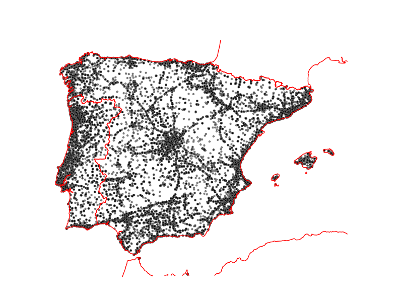
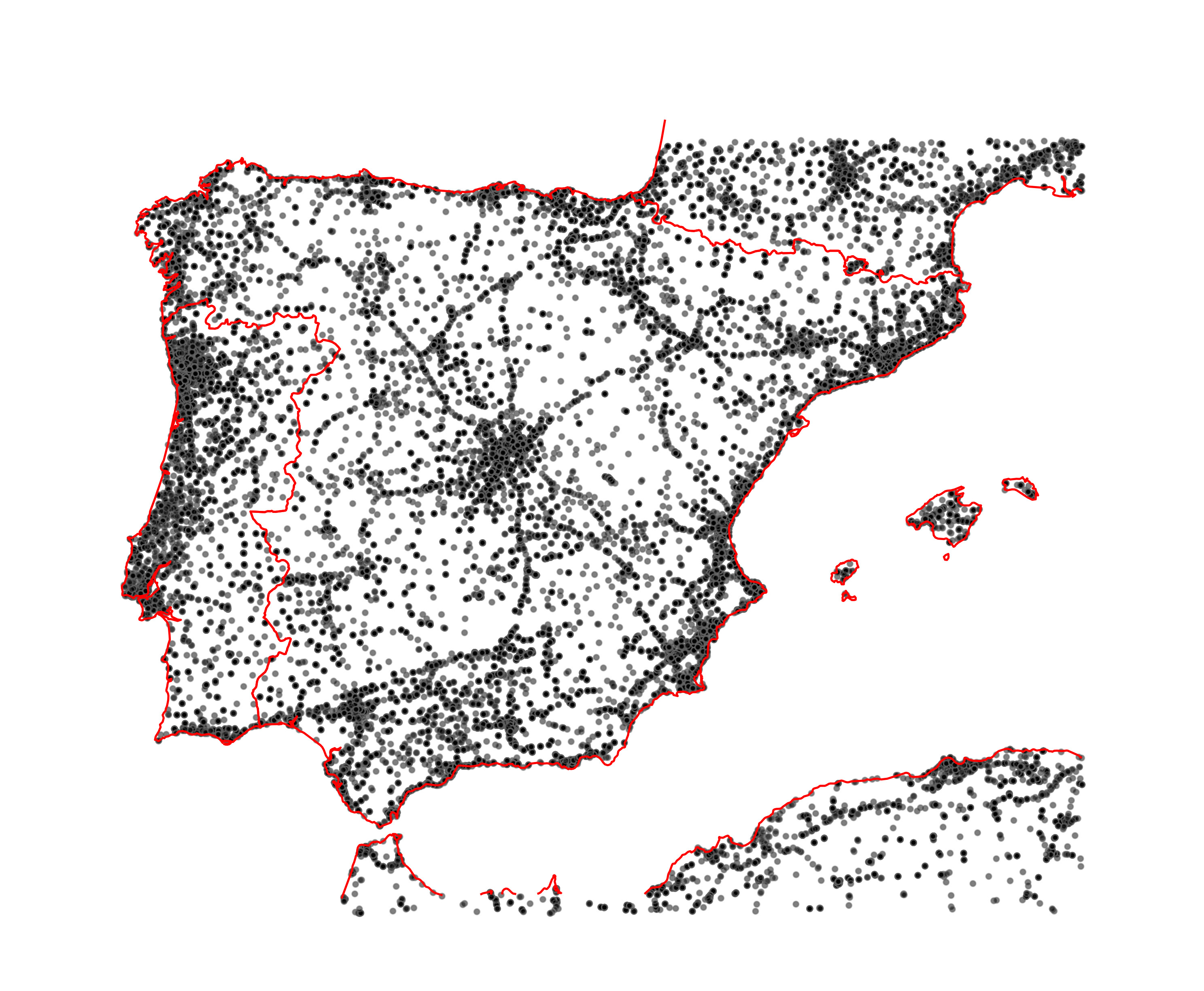
I am trying to create a graphic of the fuel stations in Iberian Peninsula (Portugal and Spain) without the islands.

For that, I use the following code in R. However, I would like to remove all fuel stations beyond these country borders ( red border in the graph). As you may see on the graph, fuel stations of North Africa and France also appear (I want to remove those).

#install the osmdata, sf, tidyverse and ggmap package
if(!require("osmdata")) install.packages("osmdata")
if(!require("tidyverse")) install.packages("tidyverse")
if(!require("sf")) install.packages("sf")
if(!require("rnaturalearth")) install.packages("rnaturalearth")

#load packages
library(tidyverse)
library(osmdata)
library(sf)
library(rnaturalearth)

# Bounding box for the Iberian Peninsula

m <- c(-10, 35, 5.0, 44)

peninsula.lim = data.frame(ylim=c(35, 44), xlim=c(-10, 5.0))

map <- ne_countries(scale = 10, returnclass = "sf") %>% st_cast("MULTILINESTRING")

map <- st_crop(map, xmin = -10, xmax = 5, ymin = 35, ymax = 44)

# building the query for fuel gas stations
# The fuel tag is used to map a fuel station, also known as a filling station
q <- m %>% 
  opq (timeout = 25*1000) %>%
  add_osm_feature("amenity", "fuel")

#query
fuel <- osmdata_sf(q)

#final map
final_fuel <- ggplot(fuel$osm_points) + 
  geom_sf(colour = "grey39",
          fill = "grey0",
          alpha = .5,
          size = 1,
          shape = 21)+
  coord_sf(ylim=peninsula.lim$ylim, xlim=peninsula.lim$xlim, expand = FALSE) +
  geom_sf(data = map, colour = "red", size = 1.0) +
  theme_void() + 
  theme(
    plot.title = element_text(face = "bold",
                              size = 22, color = "grey28",
                              hjust = .5
    ),
    plot.caption = element_text(
      size = 10,
      color = "grey28",
      margin = margin(b = 5, t = 5, unit = "pt")
    ),
    plot.margin = unit(
      c(t = 1, r = 0, l = 0, b = 0), "lines"
    )
  ) +
  labs(
    x = "",
    y = "",
    title = "",
    caption = "",
  )

plot(final_fuel)

The graphic that the above code does is as follows:

Could you please help me solve this.

Thanks,
Luis

[jlacko]

The filtering can be done by means of sf::st_within() geometric binary predicate, with sparse set to FALSE / so that it will return not a sparse matrix, but dense logical vector. Which in turn can be fed to dplyr::filter() to subset the rows of fuel stations.

In order to achieve that I had to cast your map object from linestring back to polygon, and unite the two countries of intereset. I have also moved the selection of osm_points upward in your code, from the final map to query selection.

On a personal note I have two kind of tangential observations:

• I would advise against using names of functions as object names, especially when loading {tidyverse} metapackage in as a single call - yes, purrr::map() I am looking at you! It is a naming conflict waiting to happen...
• I find it mildly amusing how the North African gasolineras disappear, except for the couple in Ceuta and Melilla

#install the osmdata, sf, tidyverse and ggmap package
if(!require("osmdata")) install.packages("osmdata")
if(!require("tidyverse")) install.packages("tidyverse")
if(!require("sf")) install.packages("sf")
if(!require("rnaturalearth")) install.packages("rnaturalearth")

#load packages
library(tidyverse)
library(osmdata)
library(sf)
library(rnaturalearth)

# Bounding box for the Iberian Peninsula

m <- c(-10, 35, 5.0, 44)

peninsula.lim = data.frame(ylim=c(35, 44), xlim=c(-10, 5.0))

map <- ne_countries(scale = 10, returnclass = "sf") %>% st_cast("MULTILINESTRING")

map <- st_crop(map, xmin = -10, xmax = 5, ymin = 35, ymax = 44)

# building the query for fuel gas stations
# The fuel tag is used to map a fuel station, also known as a filling station
q <- m %>% 
  opq (timeout = 25*1000) %>%
  add_osm_feature("amenity", "fuel")

#query
fuel <- osmdata_sf(q)$osm_points %>% 
  dplyr::filter(st_within(., subset(map, sov_a3 %in% c("ESP", "PRT")) %>% 
                            st_cast("POLYGON") %>% 
                            summarise(), 
                          sparse = F) [,1])


#final map
final_fuel <- ggplot(fuel) + 
  geom_sf(colour = "grey39",
          fill = "grey0",
          alpha = .5,
          size = 1,
          shape = 21)+
  coord_sf(ylim=peninsula.lim$ylim, xlim=peninsula.lim$xlim, expand = FALSE) +
  geom_sf(data = map, colour = "red", size = 1.0) +
  theme_void() + 
  theme(
    plot.title = element_text(face = "bold",
                              size = 22, color = "grey28",
                              hjust = .5
    ),
    plot.caption = element_text(
      size = 10,
      color = "grey28",
      margin = margin(b = 5, t = 5, unit = "pt")
    ),
    plot.margin = unit(
      c(t = 1, r = 0, l = 0, b = 0), "lines"
    )
  ) +
  labs(
    x = "",
    y = "",
    title = "",
    caption = "",
  )

plot(final_fuel)

[lbarqueira]

@jlacko Thank you very much. I learned a lot.