Reduce processing time for calculating coefficients

I have a database, a function, and from that, I can get coef value (it is calculated through lm function). There are two ways of calculating: the first is if I want a specific coefficient depending on an ID, date and Category and the other way is calculating all possible coef, according to subset_df1.

The code is working. For the first way, it is calculated instantly, but for the calculation of all coefs, it takes a reasonable amount of time, as you can see. I used the tictoc function just to show you the calculation time, which gave 633.38 sec elapsed. An important point to highlight is that df1 is not such a small database, but for the calculation of all coef I filter, which in this case is subset_df1.

I made explanations in the code so you can better understand what I'm doing. The idea is to generate coef values ​​for all dates >= to date1.

Finally, I would like to try to reasonably decrease this processing time for calculating all coef values.

library(dplyr)
library(tidyr)
library(lubridate)
library(tictoc)

#database
df1 <- data.frame( Id = rep(1:5, length=900),
                   date1 =  as.Date( "2021-12-01"),
                   date2= rep(seq( as.Date("2021-01-01"), length.out=450, by=1), each = 2),
                   Category = rep(c("ABC", "EFG"), length.out = 900),
                   Week = rep(c("Monday", "Tuesday", "Wednesday", "Thursday", "Friday",
                                "Saturday", "Sunday"), length.out = 900),
                   DR1 = sample( 200:250, 900, repl=TRUE),  
                   setNames( replicate(365, { sample(0:900, 900)}, simplify=FALSE),
                             paste0("DRM", formatC(1:365, width = 2, format = "d", flag = "0"))))
                             
return_coef <- function(df1,idd,dmda,CategoryChosse) {
  
  # First idea: Calculate the median of the values resulting from the subtraction between DR01 and the values of the DRM columns
  
  subsetDRM<-  df1 %>% select(starts_with("DRM")) 
  
  DR1_subsetDRM<-cbind (df1, setNames(df1$DR1 - subsetDRM, paste0(names(subsetDRM), "_PV"))) 
  
  subset_PV<-select(DR1_subsetDRM,Id, date2,Week, Category, DR1, ends_with("PV")) 
  
  result_median<-subset_PV %>%
    group_by(Id,Category,Week) %>%
    dplyr::summarize(dplyr::across(ends_with("PV"), median),.groups = 'drop')
  
  # Second idea: After obtaining the median, I add the values found with the values of the DRM columns of my df1 database.
  
  Sum_DRM_result_median<-df1%>%
    inner_join(result_median, by = c('Id','Category', 'Week')) %>%
    mutate(across(matches("^DRM\\d+$"), ~.x + get(paste0(cur_column(), '_PV')),
                  .names = '{col}_{col}_PV')) %>%
    select(Id:Category, DRM01_DRM01_PV:last_col())
  
  Sum_DRM_result_median<-data.frame(Sum_DRM_result_median)
  
  # Third idea: The idea here is to specifically filter a line from Sum_DRM_result_median, which will depend on what the user chooses, for that it will be necessary to choose an Id, date and Category.
  
  # This code `remove_values_0` I use because sometimes i have values equal to zero so i remove these columns   
  remove_values_0 <- df1 %>%
    dplyr::filter(Id==idd,date2 == ymd(dmda), Category == CategoryChosse) %>%
    select(starts_with("DRM")) %>%
    pivot_longer(cols = everything()) %>%
    arrange(desc(row_number())) %>%
    mutate(cs = cumsum(value)) %>%
    dplyr::filter(cs == 0) %>%
    pull(name)
  (dropnames <- paste0(remove_values_0,"_",remove_values_0, "_PV"))
  
  filterid_date_category <- Sum_DRM_result_median %>%
    filter(Id==idd,date2 == ymd(dmda), Category == CategoryChosse) %>%
    select(-any_of(dropnames))
  
  #Fourth idea: After selecting the corresponding row, I need to select the datas for coef calculation. For this, I delete some initial lines, which will depend on the day chosen.
  
  datas <-filterid_date_category %>%
    filter(Id==idd,date2 == ymd(dmda)) %>%
    group_by(Category) %>%
    summarize(across(starts_with("DRM"), sum),.groups = 'drop') %>%
    pivot_longer(cols= -Category, names_pattern = "DRM(.+)", values_to = "val") %>%
    mutate(name = readr::parse_number(name))
  colnames(datas)[-1]<-c("days","numbers")
  
  datas <- datas %>% 
    group_by(Category) %>% 
    slice((ymd(dmda) - min(as.Date(df1$date1) [
      df1$Category == first(Category)])):max(days)+1) %>%
    ungroup
  
  # After I calculate the datas dataset, I used the lm function to obtain the coef value.
  
  mod <- lm(numbers ~ I(days^2), datas)
  coef<-coef(mod)[1]
  val<-as.numeric(coef(mod)[1])
  
  return(val)
  
}

To calculate the coef of a specific ID, Date and Category in my df1 database, I do:

return_coef(df1,"2","2021-12-10","ABC")
[1] 209.262 # This value may vary, as the values ​​in my df1 database vary

To calculate all the coef, I do:

tic()
subset_df1 <- subset(df1, date2 >= date1)

All<-subset_df1%>%
   transmute(
     Id,date2,Category,
     coef = mapply(return_coef, list(cur_data()), Id, as.Date(date2), Category))
toc()
633.38 sec elapsed
Profiling with Rstudio's Profilter showed me that the slow part of your function is

dplyr::summarize(dplyr::across(ends_with("PV"), median),.groups = 'drop')

I found that this could be improved 24x with data.table and dtplyr

g1 <- subset_PV %>%
  group_by(Id,Category,Week) 

g1 %>%
  dplyr::summarize(dplyr::across(ends_with("PV"), median),.groups = 'drop')
 
library(dtplyr)
 library(data.table)

g2 <- subset_PV %>%
  group_by(Id,Category,Week) %>% lazy_dt()

g2 %>%
  dplyr::summarize(dplyr::across(ends_with("PV"), median),.groups = 'drop') %>% as_tibble()

library(bench)
bench::mark(g1_result = g1 %>%
              dplyr::summarize(dplyr::across(ends_with("PV"), median),.groups = 'drop'),
            g2_result = g2 %>%
              dplyr::summarize(dplyr::across(ends_with("PV"), median),.groups = 'drop') %>% as_tibble())

Thanks for reply @nirgrahamuk, However, when I run your code it appears: Error: Each result must equal the first result: g1_resultdoes not equalg2_result`

You copied and pasted my code or wrote it out yourself yourself ?

Hi @nirgrahamuk , so, I found it strange that g1 I get 70 obs and 368 variables and g2 I get 1 obs and 366 variables, wouldn't they have to be the same number of observations and variables? With g2 I can't calculate Sum_DRM_result_median

g1 <- subset_PV %>%
group_by(Id,Category,Week) %>%
dplyr::summarize(dplyr::across(ends_with("PV"), median),.groups = 'drop')
nrow(g1)
[1] 70


g2 <- subset_PV %>%
group_by(Id,Category,Week) %>% lazy_dt() %>%
dplyr::summarize(dplyr::across(ends_with("PV"), median),.groups = 'drop') %>% as_tibble()
nrow(g2)
 [1] 1

Sometimes, we get so caught up in how it's easy to lose track of what. To bring back the key part of analysis, it helps to recall basic algebra from school days: f(x)=y.

x is df1, the data at hand.
y is the desired output, an object containing the coefficients of linear regressions.

What is the data argument to lm? A subset of df1.
What is the formula argument to lm? The median value of the DRM values of df1 against the square of days elapsed between date1 and date2.

Leaving aside how to create the subset and collect the coefficient results of the linear regression, consider the following:

a <- data.frame(sqr = 111556, med = 433)
lm(med ~ sqr, data = a) |> summary()
#> 
#> Call:
#> lm(formula = med ~ sqr, data = a)
#> 
#> Residuals:
#> ALL 1 residuals are 0: no residual degrees of freedom!
#> 
#> Coefficients: (1 not defined because of singularities)
#>             Estimate Std. Error t value Pr(>|t|)
#> (Intercept)      433        NaN     NaN      NaN
#> sqr               NA         NA      NA       NA
#> 
#> Residual standard error: NaN on 0 degrees of freedom

appears equivalent, selecting a single row, deriving a median value for the DRM variables and the square of the elapsed days.

Efficiency is besides the point here.

library(ggplot2)
library(lubridate)
#> 
#> Attaching package: 'lubridate'
#> The following objects are masked from 'package:base':
#> 
#>     date, intersect, setdiff, union

# database
df1 <- data.frame(
  Id = rep(1:5, length = 900),
  date1 = as.Date("2021-12-01"),
  date2 = rep(seq(as.Date("2021-01-01"), length.out = 450, by = 1), each = 2),
  Category = rep(c("ABC", "EFG"), length.out = 900),
  Week = rep(c(
    "Monday", "Tuesday", "Wednesday", "Thursday", "Friday",
    "Saturday", "Sunday"
  ), length.out = 900),
  DR1 = sample(200:250, 900, repl = TRUE),
  setNames(
    replicate(365,
      {
        sample(0:900, 900)
      },
      simplify = FALSE
    ),
    paste0("DRM", formatC(1:365, width = 2, format = "d", flag = "0"))
  )
)


filter_dates <- function(x) x[which(x[,2] >= x[,3]),]
get_days_sq <- function(x) x$days = as.numeric(x$date1 - x$date2)^2
pick_drm <- function(x) x[,7:length(x)]

a <- filter_dates(df1)
b <- pick_drm(a)
d <- get_days_sq(a)
e <- apply(b[,1:365],1,median)
b$sqr <- d
b$med <- e
cat1 <- which(a$Category == "ABC")
cat2 <- which(a$Category == "EFG")

# visualize
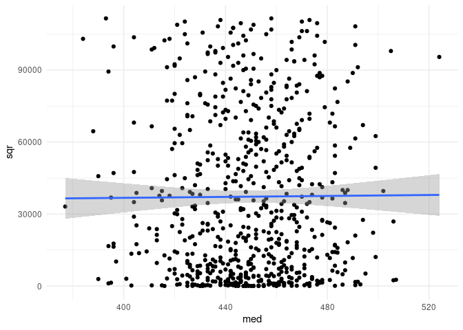
ggplot(b,aes(med,sqr)) + geom_point() + geom_smooth(method  = "lm") + theme_minimal()
#> `geom_smooth()` using formula 'y ~ x'

f <- lm(med ~ sqr, data = b[1,]) # attempt to regress on two numeric values
summary(f)
#> 
#> Call:
#> lm(formula = med ~ sqr, data = b[1, ])
#> 
#> Residuals:
#> ALL 1 residuals are 0: no residual degrees of freedom!
#> 
#> Coefficients: (1 not defined because of singularities)
#>             Estimate Std. Error t value Pr(>|t|)
#> (Intercept)      393        NaN     NaN      NaN
#> sqr               NA         NA      NA       NA
#> 
#> Residual standard error: NaN on 0 degrees of freedom

# regress by Category variable

ABC <- b[cat1,]
EFG <- b[cat2,]

# this returns an lm model
f1 <- lm(med ~ sqr, data = ABC)
summary(f1)
#> 
#> Call:
#> lm(formula = med ~ sqr, data = ABC)
#> 
#> Residuals:
#>     Min      1Q  Median      3Q     Max 
#> -72.510 -14.728   0.288  17.029  58.227 
#> 
#> Coefficients:
#>              Estimate Std. Error t value Pr(>|t|)    
#> (Intercept) 4.487e+02  1.932e+00 232.293   <2e-16 ***
#> sqr         2.415e-05  3.863e-05   0.625    0.532    
#> ---
#> Signif. codes:  0 '***' 0.001 '**' 0.01 '*' 0.05 '.' 0.1 ' ' 1
#> 
#> Residual standard error: 23.59 on 333 degrees of freedom
#> Multiple R-squared:  0.001172,   Adjusted R-squared:  -0.001828 
#> F-statistic: 0.3907 on 1 and 333 DF,  p-value: 0.5324

# the coefficient
coef(f1)[2]
#>          sqr 
#> 2.414616e-05

# this returns an lm model
f2 <- lm(med ~ sqr, data = ABC)
summary(f2)
#> 
#> Call:
#> lm(formula = med ~ sqr, data = ABC)
#> 
#> Residuals:
#>     Min      1Q  Median      3Q     Max 
#> -72.510 -14.728   0.288  17.029  58.227 
#> 
#> Coefficients:
#>              Estimate Std. Error t value Pr(>|t|)    
#> (Intercept) 4.487e+02  1.932e+00 232.293   <2e-16 ***
#> sqr         2.415e-05  3.863e-05   0.625    0.532    
#> ---
#> Signif. codes:  0 '***' 0.001 '**' 0.01 '*' 0.05 '.' 0.1 ' ' 1
#> 
#> Residual standard error: 23.59 on 333 degrees of freedom
#> Multiple R-squared:  0.001172,   Adjusted R-squared:  -0.001828 
#> F-statistic: 0.3907 on 1 and 333 DF,  p-value: 0.5324

# the coefficient
coef(f2)[2]
#>          sqr 
#> 2.414616e-05

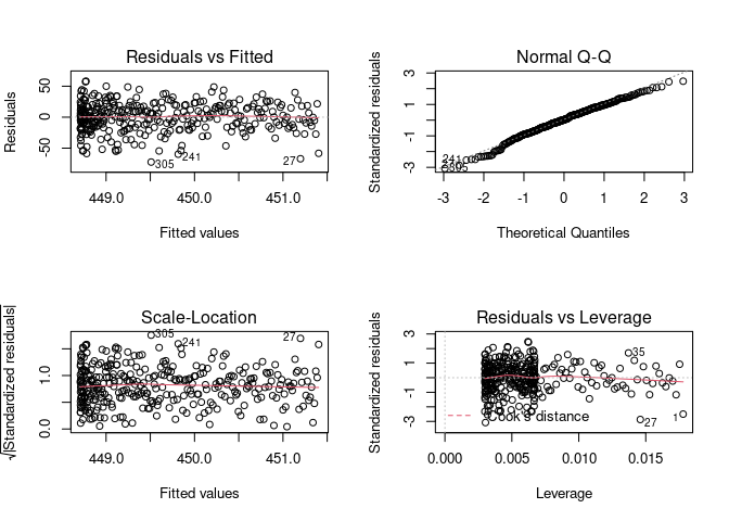
# diagnostic plots
par(mfrow = c(2,2))
plot(f1)
plot(f2)

This topic was automatically closed 21 days after the last reply. New replies are no longer allowed.

If you have a query related to it or one of the replies, start a new topic and refer back with a link.