Hello,
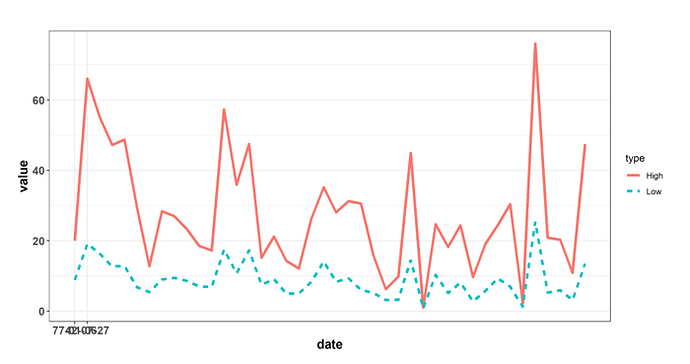
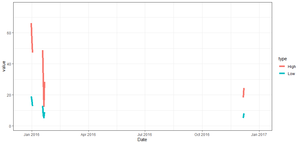
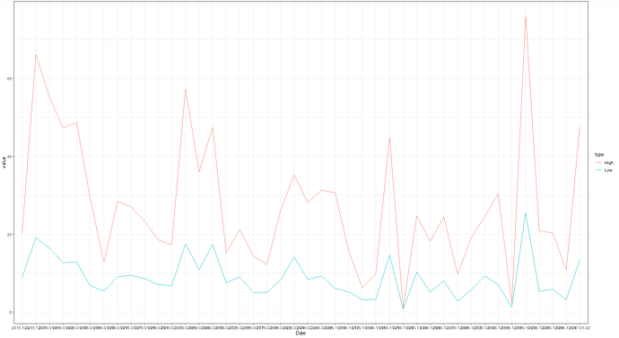
I would reconsidering using bdscale. Do you really need this package? Not sure it brings you any value. In the code below you will see you data transformed into a tsibble, or time series tibble, and use the tsibble package to test for things that matter for time series like missing time gaps. The last graph has your data with NA's filled in for the missing weeks. Like @EconProf said, you are missing a lot of data between observations.
R has some great packages for time series, tsibble being one, and the fable packages for time series modeling. The learning curve can be large sometimes, but it will be worth it in the end. Welcome to R!
library(tidyverse)
library(bdscale)
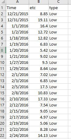
time_dta <- as.data.frame(
  list(Time = c("12/21/2015", "12/31/2015", "1/1/2016",
                "1/2/2016", "1/18/2016", "1/19/2016", "1/20/2016", "1/21/2016",
                "1/27/2016", "1/29/2016", "2/1/2016", "2/3/2016", "2/5/2016",
                "2/8/2016", "2/10/2016", "2/12/2016", "2/15/2016", "2/17/2016",
                "2/19/2016", "2/22/2016", "2/24/2016", "2/26/2016", "2/29/2016",
                "11/10/2016", "11/12/2016", "11/14/2016", "11/16/2016", "11/25/2016",
                "11/28/2016", "11/30/2016", "12/6/2016", "12/7/2016", "12/9/2016",
                "12/12/2016", "12/14/2016", "12/16/2016", "12/19/2016", "12/23/2016",
                "12/26/2016", "12/28/2016", "12/30/2016", "1/2/2017", "12/21/2015",
                "12/31/2015", "1/1/2016", "1/2/2016", "1/18/2016", "1/19/2016",
                "1/20/2016", "1/21/2016", "1/27/2016", "1/29/2016", "2/1/2016",
                "2/3/2016", "2/5/2016", "2/8/2016", "2/10/2016", "2/12/2016",
                "2/15/2016", "2/17/2016", "2/19/2016", "2/22/2016", "2/24/2016",
                "2/26/2016", "2/29/2016", "11/10/2016", "11/12/2016", "11/14/2016",
                "11/16/2016", "11/25/2016", "11/28/2016", "11/30/2016", "12/6/2016",
                "12/7/2016", "12/9/2016", "12/12/2016", "12/14/2016", "12/16/2016",
                "12/19/2016", "12/23/2016", "12/26/2016", "12/28/2016", "12/30/2016",
                "1/2/2017"), etc = c(8.85, 19.11, 16.4, 12.72, 12.82, 6.83, 5.42,
                                     9.02, 9.5, 8.64, 7.02, 6.85, 17.5, 10.83, 17.33, 7.54, 9.05,
                                     4.97, 5.06, 8.28, 14.13, 8.38, 9.28, 6.05, 5.2, 3.17, 3.22, 14.63,
                                     0.81, 10.29, 5.17, 8.09, 2.77, 5.76, 9.29, 6.96, 1.27, 25.46,
                                     5.29, 5.92, 3.2, 13.5, 20.09, 66.11, 55.21, 47.24, 48.71, 29.32,
                                     12.74, 28.39, 27.03, 23.35, 18.58, 17.27, 57.33, 35.9, 47.47,
                                     15.17, 21.22, 14.31, 12.15, 26.17, 35.19, 28.08, 31.27, 30.61,
                                     15.74, 6.22, 9.8, 44.9, 1.02, 24.72, 18.23, 24.42, 9.68, 19.05,
                                     24.53, 30.37, 2.28, 75.95, 20.86, 20.32, 10.89, 47.49), type = c("Low",
                                                                                                      "Low", "Low", "Low", "Low", "Low", "Low", "Low", "Low", "Low",
                                                                                                      "Low", "Low", "Low", "Low", "Low", "Low", "Low", "Low", "Low",
                                                                                                      "Low", "Low", "Low", "Low", "Low", "Low", "Low", "Low", "Low",
                                                                                                      "Low", "Low", "Low", "Low", "Low", "Low", "Low", "Low", "Low",
                                                                                                      "Low", "Low", "Low", "Low", "Low", "High", "High", "High", "High",
                                                                                                      "High", "High", "High", "High", "High", "High", "High", "High",
                                                                                                      "High", "High", "High", "High", "High", "High", "High", "High",
                                                                                                      "High", "High", "High", "High", "High", "High", "High", "High",
                                                                                                      "High", "High", "High", "High", "High", "High", "High", "High",
                                                                                                      "High", "High", "High", "High", "High", "High"))
)

str(time_dta)
as.character(trimws(time_dta$Time)) %>% str()
time_dta <- time_dta %>%
  mutate(date_str = as.character(.data$Time),
         date = as.Date(date_str, format = '%m/%d/%Y'))

str(time_dta)

time_ts <- tsibble::tsibble(time_dta, key = type, index = date)
str(time_ts)
tsibble::key(time_ts)
tsibble::index(time_ts)

# Your data has duplicates because you have High and Low
tsibble::is_duplicated(time_ts)
tsibble::are_duplicated(time_ts)

time_ts <- time_ts %>% tsibble::group_by_key(.data$type)

# Your data has duplicates because you have High and Low and NA's
tsibble::duplicates(time_ts)
tsibble::is_duplicated(time_ts)
tsibble::are_duplicated(time_ts)

tsibble::has_gaps(time_ts)

time_ts %>% ggplot(aes(x=date,y=etc, color=type)) +
  xlab("Date") +
  ylab("value") +
  geom_line() +
  #scale_x_bd(business.dates=date, labels = date_format("%Y-%m-%d"), max.major.breaks=100) +
  theme_bw()

time_ts_complete <- tsibble::fill_gaps(time_ts)

tsibble::duplicates(time_ts_complete)
tsibble::is_duplicated(time_ts_complete)
tsibble::are_duplicated(time_ts_complete)

time_ts_complete %>% ggplot(aes(x=date,y=etc, color=type)) +
  xlab("Date") +
  ylab("value") +
  geom_line(size = 2) +
  #scale_x_bd(business.dates=data$Time, labels = date_format("%Y-%m-%d"), max.major.breaks=100)+
  theme_bw()


 .
.