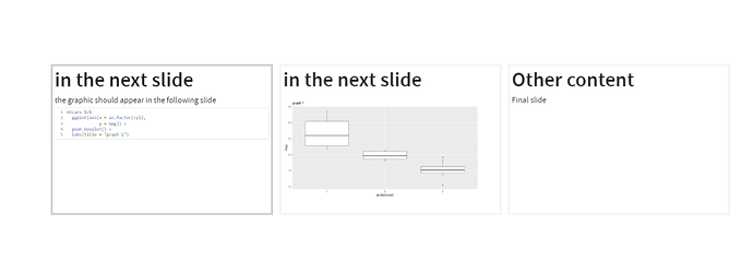
which is what I expect
- code 1
- figure 1
- code 2
- figure 2
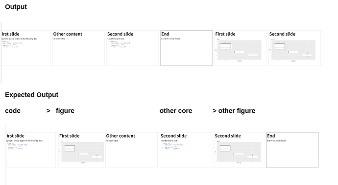
what happens
- code 1
- code 2
- figure 1
- figure 2
Check this code and slides
---
title: "Test"

execute:
  echo: true
  warning: false
format:
  revealjs:
    slide-number: true
---

```{r}
#if not installed, run next line
# install.packages("pacman")
pacman::p_load(tidyverse)
```


## Hello, There

This presentation will show you examples of what you can do with Quarto and [Reveal.js](https://revealjs.com), including:

-   Presenting code and LaTeX equations
-   Including computations in slide output
-   Image, video, and iframe backgrounds
-   Fancy transitions and animations
-   Printing to PDF

...and much more

## a code

```{r}
glimpse(mtcars)
```
## a plot
```{r}
mtcars %>%
  ggplot(aes(x = as.factor(cyl),
             y = mpg)) +
  geom_boxplot()

```
# in the same slide
```{r}
#| output-location: fragment
mtcars %>%
  ggplot(aes(x = as.factor(cyl),
             y = mpg)) +
  geom_boxplot()

```

# in the next slide
the graphic should appear in the following slide
```{r}
#| output-location: slide
mtcars %>%
  ggplot(aes(x = as.factor(cyl),
             y = mpg)) +
  geom_boxplot() +
  labs(title = "graph 1")

```

# in the next slide 2
the graphic should appear in the following slide
```{r}
#| output-location: slide
mtcars %>%
  ggplot(aes(x = as.factor(cyl),
             y = mpg)) +
  geom_boxplot() +
  labs(title = "graph 2")

```

# Mixed


# in the next slide
the graphic should appear in the following slide
```{r}
#| output-location: slide
mtcars %>%
  ggplot(aes(x = as.factor(cyl),
             y = mpg)) +
  geom_boxplot() +
  labs(title = "graph 3")

```

# in the same slide
```{r}
#| output-location: fragment
mtcars %>%
  ggplot(aes(x = as.factor(cyl),
             y = mpg)) +
  geom_boxplot()

```

# in the next slide 4
the graphic should appear in the following slide
```{r}
#| output-location: slide
mtcars %>%
  ggplot(aes(x = as.factor(cyl),
             y = mpg)) +
  geom_boxplot() +
  labs(title = "graph 4")
```

