Proportional odds assumption in R

Hi!
For my thesis I use a cumulative link model to explore correlations between ordinal data (likert-scale) and continious data. One of the assumptions is the proportional odds assumption.
I did find that R doesn't have a good test for this. However, there is a graphical way according to Harrell (Harrell 2001 p 335). This method is explaind here:
Ordinal Logistic Regression | R Data Analysis Examples under the proportional odds assumption title...
I tried this method on my data, but I only get 'errors'... someone who knows what goes wrong?

Dataset

Sub Groep Niet_Behandeling 2.1 2.2 2.3 2.4 2.5 2.6 2.7 2.8 2.9 2.10 2.11 2.12 2.13 2.14 2.15 2.16 2.17 2.18
1 1 BE 1 2 1 4 2 1 3 3 4 1 1 1 1 1 1 1 3 1 3
2 23 BE 1 2 4 2 1 1 1 2 4 1 1 1 1 5 1 1 1 1 4
3 24 BE 1 1 4 2 1 1 1 1 1 1 1 1 1 1 1 1 1 1 4
4 25 BEBD 1 2 2 4 2 2 2 4 4 3 3 3 3 3 3 3 3 3 4
5 27 BE 1 2 3 4 1 3 4 1 4 2 4 1 1 1 1 1 1 1 1
6 32 BEBD 1 1 4 2 4 1 4 1 4 1 5 1 3 1 1 1 1 1 1
7 34 BE 1 2 5 4 4 4 3 4 4 4 3 3 3 3 2 1 3 3 3
8 37 BE 1 3 3 4 2 1 3 2 2 3 1 1 1 3 1 1 1 1 1
9 38 BE 1 4 5 1 3 2 4 4 4 1 1 3 2 1 1 1 4 4 5
10 41 BE 1 3 3 3 2 2 4 4 3 2 2 2 2 2 1 1 1 1 1
11 45 BE 1 1 5 3 3 1 2 4 5 3 2 2 3 2 2 1 4 3 3
12 55 BEBD 1 1 1 1 1 1 3 2 4 1 4 1 1 5 1 1 1 1 1
13 58 BE 1 4 3 4 2 3 2 2 3 1 2 1 3 2 1 1 2 1 1
14 65 BEBD 1 4 2 5 1 1 3 2 3 1 1 1 1 1 1 1 1 1 1
15 66 BE 1 4 5 4 2 1 2 3 2 1 1 1 1 1 1 1 1 1 2
16 68 BE 1 4 2 4 5 3 4 4 3 2 2 2 2 2 1 1 2 2 3
17 72 BEBD 1 4 2 5 1 1 1 1 3 1 1 1 1 1 1 1 2 1 1
18 73 BEBD 1 4 2 4 3 2 2 2 4 1 2 2 1 2 1 1 2 1 1
2.19 2.20 2.21 2.22 EDE_Q_EC EDE_R EDE-Q_WC EDE_Q_SC EDE_Q_Totaal
1 4 3 5 3 4.8 5.6 6.0 3.750 5.03750
2 1 1 2 4 1.0 2.0 1.6 1.625 1.55625
3 3 2 1 1 4.6 5.6 6.0 6.000 5.55000
4 4 3 4 3 4.4 3.4 9.6 3.750 5.28750
5 1 1 2 1 4.6 3.4 5.8 5.875 4.91875
6 1 4 2 1 2.0 0.4 3.2 4.250 2.46250
7 3 3 4 3 3.4 1.2 5.4 5.625 3.90625
8 1 1 3 3 0.8 0.6 3.6 4.375 2.34375
9 4 4 1 1 3.2 2.0 5.8 6.000 4.25000
10 1 1 1 1 0.8 0.8 0.4 0.625 0.65625
11 5 4 4 3 3.8 2.4 5.0 5.000 4.05000
12 3 1 5 1 3.8 5.4 6.0 6.000 5.30000
13 1 3 4 3 2.2 2.8 5.0 4.750 3.68750
14 2 3 5 3 3.4 2.2 4.2 4.750 3.63750
15 2 1 5 3 1.4 3.0 2.6 3.500 2.62500
16 4 4 5 1 3.0 3.6 5.4 5.375 4.34375
17 1 1 4 3 0.8 3.0 2.8 1.625 2.05625
18 3 2 5 3 0.8 0.6 2.2 2.750 1.58750

#functie maken
sf <- function('y'){c('Y>=1' = qlogis(mean(y >= 1)),
'Y>=2' = qlogis(mean(y >= 2)),
'Y>=3' = qlogis(mean(y >= 3)),
'Y>=4' = qlogis(mean(y >= 4)),
'Y>=5' = qlogis(mean(y >= 5)))}
#functie toepassen voor de predictors
require(foreign)
require(ggplot2)
require(MASS)
require(Hmisc)
require(reshape2)

(s <- with(Dataset, summary(as.numeric('2.1') ~ 'EDE_Q_EC', fun = sf)))

(s <- with(Dataset, summary(as.numeric('2.1') ~ 'EDE_Q_EC', fun = sf)))
Error in terms.formula(formula, "stratify") :
invalid model formula in ExtractVars
Your data and code is badly readable.
Maybe that improves if you make a reprex . Search for reprex with the search option on this page.

However I think that I see that Dataset has columns/fields that have numbers as column names.
This type of name is non-standard and in that case need back-ticks around the name when you use them.
See e.g.

df = data.frame(
  `2.1` = c(1,2,3),
  `2.2` = c(200,300,400)
)
names(df) = substr(names(df),2,4)
df
#>   2.1 2.2
#> 1   1 200
#> 2   2 300
#> 3   3 400

with(df,sum('2.1'))
#> Error in sum("2.1"): invalid 'type' (character) of argument
with(df,sum(`2.1`))
#> [1] 6

Created on 2020-06-09 by the reprex package (v0.3.0)

Maybe this helps. If not it would be helpful if we could use the dataset Dataset .
The line that is in error only uses the variables 2.1 and EDE_Q_EC as I inderstand (?)

I read it in as 'numeric' because otherwise I got an error when I wanted to calculate the median and IQR, because R didn't read my data as numeric... Could it help if I didn't read the data in as 'numeric' for this part?
I need to control the correlation for 2.1-2.22 with each EDE subtype, so I will need to control this assumption for each of 2.1-2.22 with each EDE subtype I guess?
But I only tried it for 2.1 and EDE-Q-EC for the moment....

My advice: first make sure that you get the data in R in the format you need.
Only after that you do your analysis.
This also will make your code much better understandable.

Check out the documentation to find the R functions that are most suitable to read your particular input.

Thanks for the answer!
it worked when I used the back-ticks...
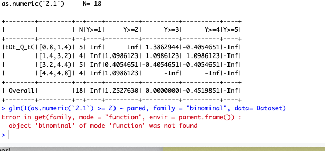
However, now I get en 'error' in the next step....
Any idea what the problem is?

#functie maken
sf <- function('y'){c('Y>=1' = qlogis(mean(y >= 1)),
'Y>=2' = qlogis(mean(y >= 2)),
'Y>=3' = qlogis(mean(y >= 3)),
'Y>=4' = qlogis(mean(y >= 4)),
'Y>=5' = qlogis(mean(y >= 5)))}

#functie toepassen voor de predictors
require(foreign)
require(ggplot2)
require(MASS)
require(Hmisc)
require(reshape2)

(s <- with(Dataset, summary(as.numeric(2.1) ~ EDE_Q_EC, fun = sf)))
s

glm(I(as.numeric(2.1) >= 2) ~ pared, family = "binominal", data= Dataset)

I uploaded a screenshot from the R-studio output...

I recognize the word binominal because I am a native Dutch speaker.
In the webpage that you are citing they use a different spelling.
Probably their mistake :wink:

I see that you did not take my advice to first ensure that the data is in good order before doing any analysis. Of course your choice ...

Well, it's not that I didn't want to follow your advise ofcourse!
It's just that when I first read in my data to calculate the median, I always got an error. So I didn't know what was wrong. When I asked help for that, they said I did need to read the data in as numeric. So, when I did that, it worked... I'm just really new to R and I don't know in which way I need to read in my data so it's in the wright order, that is why I didn't do it....