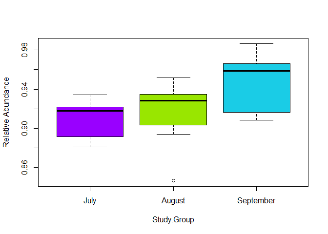
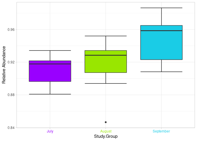
Hello everyone, I hope you and your family are very well. For some reason, due to the way I wrote this script, I have problems generating the legend of the graph that indicates the months with their respective colors.
library(readxl)
library(tibble)
library(dplyr)
#>
#> Attaching package: 'dplyr'
#> The following objects are masked from 'package:stats':
#>
#>     filter, lag
#> The following objects are masked from 'package:base':
#>
#>     intersect, setdiff, setequal, union
library(writexl)
require(car)
#> Loading required package: car
#> Loading required package: carData
#>
#> Attaching package: 'car'
#> The following object is masked from 'package:dplyr':
#>
#>     recode
library(ggplot2)
library(qqplotr)
#>
#> Attaching package: 'qqplotr'
#> The following objects are masked from 'package:ggplot2':
#>
#>     stat_qq_line, StatQqLine
library(DescTools)
#>
#> Attaching package: 'DescTools'
#> The following object is masked from 'package:car':
#>
#>     Recode
library(FSA)
#> Registered S3 methods overwritten by 'FSA':
#>   method       from
#>   confint.boot car
#>   hist.boot    car
#> ## FSA v0.9.1. See citation('FSA') if used in publication.
#> ## Run fishR() for related website and fishR('IFAR') for related book.
#>
#> Attaching package: 'FSA'
#> The following object is masked from 'package:car':
#>
#>     bootCase
library(PMCMRplus)

#Domains <- read_excel("~/RSTUDIO/Domains.xlsx")
Domains  <- data.frame (tibble::tribble(
                           ~Study.Group,     ~Domains,   ~Bacteria,    ~Archaea,    ~Eukarya,      ~Virus,
                                 "July", "61_contigs", 0.880847116, 0.002643801, 0.115560065, 0.000949017,
                                 "July", "62_contigs", 0.920484467, 0.005188828, 0.072881856, 0.001444848,
                                 "July", "63_contigs", 0.925870536, 0.005730109, 0.066773145,  0.00162621,
                                 "July", "64_contigs", 0.890393147, 0.005825359, 0.102438051, 0.001343443,
                                 "July", "65_contigs", 0.891769753, 0.003653817, 0.103614837, 0.000961593,
                                 "July", "66_contigs", 0.922044928, 0.005587012, 0.070744779, 0.001623281,
                                 "July", "67_contigs", 0.917569758, 0.005504784, 0.075590999,  0.00133446,
                                 "July", "68_contigs", 0.910076424, 0.005385183, 0.083217084, 0.001321309,
                                 "July", "69_contigs", 0.934224313, 0.007010934,  0.05702881, 0.001735942,
                                 "July", "70_contigs", 0.918057364, 0.006857865, 0.073332504, 0.001752268,
                               "August", "71_contigs", 0.933091981, 0.006099055, 0.058892902, 0.001916062,
                               "August", "72_contigs", 0.919146441, 0.005529882, 0.074240681, 0.001082996,
                               "August", "73_contigs", 0.939901124, 0.007186859, 0.051068078, 0.001843938,
                               "August", "74_contigs", 0.893910442,  0.00553633, 0.099356539, 0.001196689,
                               "August", "75_contigs", 0.846584608,  0.00304495, 0.149613348, 0.000757093,
                               "August", "76_contigs", 0.923791063, 0.003430949, 0.072009401, 0.000768587,
                               "August", "77_contigs", 0.933076213, 0.006284349, 0.058913334, 0.001726104,
                               "August", "78_contigs", 0.903286566, 0.005218661, 0.090166915, 0.001327858,
                               "August", "79_contigs", 0.951990696, 0.006367051, 0.039858017, 0.001784236,
                               "August", "80_contigs", 0.934641791, 0.005916396, 0.056694205, 0.002747607,
                            "September", "81_contigs", 0.942534071, 0.006531338, 0.049154322, 0.001780269,
                            "September", "82_contigs",  0.96629261, 0.005941053, 0.026163694, 0.001602643,
                            "September", "83_contigs", 0.960738692, 0.005542873, 0.032279947, 0.001438487,
                            "September", "84_contigs", 0.916569098, 0.004954535, 0.077039878, 0.001436489,
                            "September", "85_contigs", 0.914282139, 0.006007411, 0.078013275, 0.001697175,
                            "September", "86_contigs",    0.973336, 0.003445779, 0.022345596, 0.000872625,
                            "September", "87_contigs", 0.959918428,    0.006089,  0.03207625, 0.001916321,
                            "September", "88_contigs", 0.908228318, 0.003879184, 0.086912551, 0.000979946,
                            "September", "89_contigs",  0.98637235, 0.005068201, 0.007204716, 0.001354733,
                            "September", "90_contigs",  0.95708559, 0.007037582, 0.033863142, 0.002013686
                           )
)

July <- Domains %>% slice(1:10)
August <- Domains %>% slice(11:20)
September <- Domains %>% slice(21:30)


Bacteria <- tibble("Jul" = July$Bacteria, "Aug" = August$Bacteria, "Sep" = September$Bacteria)
Eukarya <- tibble("Jul" = July$Eukarya, "Aug" = August$Eukarya, "Sep" = September$Eukarya)
Archaea <- tibble("Jul" = July$Archaea, "Aug" = August$Archaea, "Sep" = September$Archaea)
Virus <- tibble("Jul" = July$Virus, "Aug" = August$Virus, "Sep" = September$Virus)


BacteriaRA <- data.frame(x=unlist(Bacteria))
Bacteria2 <- tibble("Study.Group" = Domains$`Study.Group`, "Bacteria" = BacteriaRA$x)
ArchaeaRA <- data.frame(x=unlist(Archaea))
Archaea2 <- tibble("Study.Group" = Domains$`Study.Group`, "Archaea" = ArchaeaRA$x)
EukaryaRA <- data.frame(x=unlist(Eukarya))
Eukarya2 <- tibble("Study.Group" = Domains$`Study.Group`, "Eukarya" = EukaryaRA$x)
VirusRA <- data.frame(x=unlist(Virus))
Virus2 <- tibble("Study.Group" = Domains$`Study.Group`, "Virus" = VirusRA$x)


shapiro.test(Bacteria$Jul)
#>
#>  Shapiro-Wilk normality test
#>
#> data:  Bacteria$Jul
#> W = 0.90555, p-value = 0.2518
shapiro.test(Bacteria$Aug)
#>
#>  Shapiro-Wilk normality test
#>
#> data:  Bacteria$Aug
#> W = 0.85853, p-value = 0.07331
shapiro.test(Bacteria$Sep)
#>
#>  Shapiro-Wilk normality test
#>
#> data:  Bacteria$Sep
#> W = 0.90877, p-value = 0.2727

fligner.test(`Bacteria` ~ `Study.Group`,Bacteria2)
#>
#>  Fligner-Killeen test of homogeneity of variances
#>
#> data:  Bacteria by Study.Group
#> Fligner-Killeen:med chi-squared = 1.2436, df = 2, p-value = 0.537
# If the test reveals a p-value greater than 0.05, indicating that there is no significant difference between the group variances
leveneTest(`Bacteria` ~ `Study.Group`,Bacteria2,center = "median")
#> Warning in leveneTest.default(y = y, group = group, ...): group coerced to
#> factor.
#> Levene's Test for Homogeneity of Variance (center = "median")
#>       Df F value Pr(>F)
#> group  2  0.5374 0.5904
#>       27
# If the test reveals a p-value greater than 0.05, indicating that there is no significant difference between the group variances

anova_bacteria <- aov(Bacteria2$Bacteria ~ Bacteria2$`Study.Group`)
summary(anova_bacteria)
#>                       Df   Sum Sq  Mean Sq F value  Pr(>F)
#> Bacteria2$Study.Group  2 0.007937 0.003969   6.075 0.00663 **
#> Residuals             27 0.017638 0.000653
#> ---
#> Signif. codes:  0 '***' 0.001 '**' 0.01 '*' 0.05 '.' 0.1 ' ' 1

# Prepare a vector of colors with specific color
my_colors <- c(
  rgb(0.6,0,1),
  rgb(0.6,0.9,0),
  rgb(0.1,0.8,0.9,maxColorValue = 1))

Bacteria2$`Study.Group` <- factor(Bacteria2$`Study.Group`,
    levels = c('July','August','September'),ordered = TRUE)

# Build the plot
boxplot(Bacteria2$Bacteria ~ Bacteria2$`Study.Group` ,
    col=my_colors,
    ylab="Relative Abundance" , xlab="Study.Group")

Created on 2021-11-26 by the reprex package (v2.0.1)

