Problem with effect size function

[rsoto310790]

Hi,

I don't understand what's wrong with the cohen.d() function to calculate the effect size. Running the function on a different data frame runs OK, there seems to be a problem with the factor levels. The output of the function suggest there's more than 2 levels in the "cut" factor variable, but there's only 2!

Any help on this?

Thanks!

Ramon

code:

#create subset dataframe

library(tidyverse)
diamonds= as.data.frame(diamonds)
diamonds_1= diamonds %>% filter(cut== "Ideal" | cut=="Fair")

#check model assumptions
#normality

ggplot(diamonds_1, aes(carat)) + geom_histogram(aes(y=..density.., color=cut)) + facet_grid(.~ cut)
#> `stat_bin()` using `bins = 30`. Pick better value with `binwidth`.

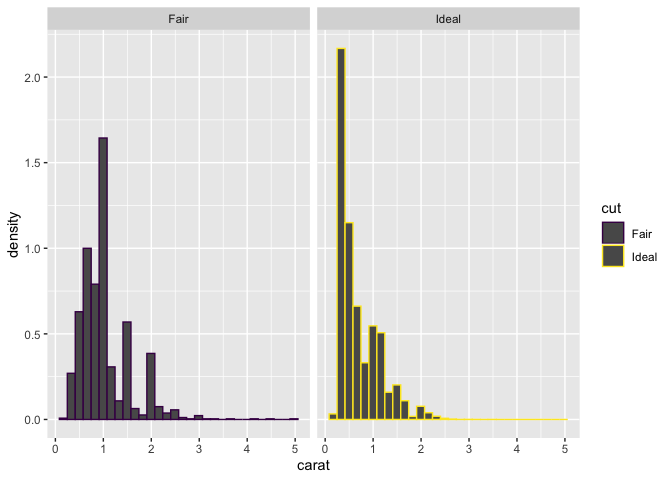
#normality is not present, but having such a big sample 
#size we can apply the central limit theorem and run the test anyway

#assumptions homogeneity of variance
library(gridExtra)
#> 
#> Attaching package: 'gridExtra'
#> The following object is masked from 'package:dplyr':
#> 
#>     combine
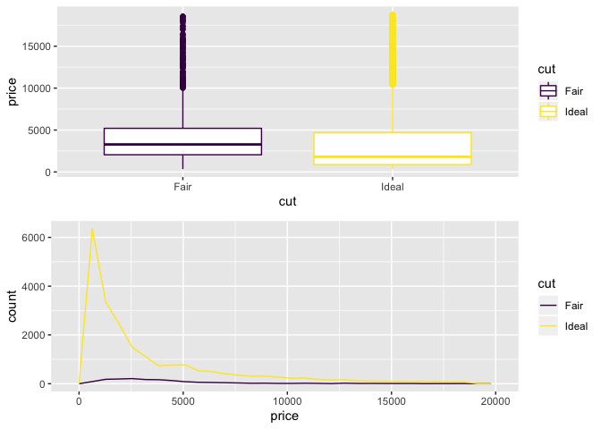
box_plot=ggplot(diamonds_1, aes(cut, price)) + geom_boxplot(aes(color=cut))
freq_poly=ggplot(diamonds_1, aes(price)) + geom_freqpoly(aes(color=cut))
grid.arrange(box_plot, freq_poly)
#> `stat_bin()` using `bins = 30`. Pick better value with `binwidth`.

fligner.test(price ~ cut, data = diamonds_1)
#> 
#>  Fligner-Killeen test of homogeneity of variances
#> 
#> data:  price by cut
#> Fligner-Killeen:med chi-squared = 7.5966, df = 1, p-value = 0.005848
#scatter on both groups seems bordelinish, depends on the significance level. we can run a test to verify this


t.test(diamonds_1[diamonds_1$cut=="Ideal", "price"], y=diamonds_1[diamonds_1$cut=="Fair", "price"], alternative = "two.sided", conf.level = 0.95, var.equal = TRUE)
#> 
#>  Two Sample t-test
#> 
#> data:  diamonds_1[diamonds_1$cut == "Ideal", "price"] and diamonds_1[diamonds_1$cut == "Fair", "price"]
#> t = -9.1995, df = 23159, p-value < 2.2e-16
#> alternative hypothesis: true difference in means is not equal to 0
#> 95 percent confidence interval:
#>  -1093.2312  -709.2004
#> sample estimates:
#> mean of x mean of y 
#>  3457.542  4358.758
t.test(diamonds_1[diamonds_1$cut=="Ideal", "price"], y=diamonds_1[diamonds_1$cut=="Fair", "price"], alternative = "two.sided", conf.level = 0.95, var.equal = FALSE)
#> 
#>  Welch Two Sample t-test
#> 
#> data:  diamonds_1[diamonds_1$cut == "Ideal", "price"] and diamonds_1[diamonds_1$cut == "Fair", "price"]
#> t = -9.7484, df = 1894.8, p-value < 2.2e-16
#> alternative hypothesis: true difference in means is not equal to 0
#> 95 percent confidence interval:
#>  -1082.5251  -719.9065
#> sample estimates:
#> mean of x mean of y 
#>  3457.542  4358.758

#both seem highly significant, indicating that the difference in the mean between the two groups is not due to chance

#calculating effect size
library(effsize)
cohen.d(formula= price ~ cut, data=diamonds_1, paired = FALSE)
#> Warning in cohen.d.default(d, f, ...): Factor with multiple levles, using only
#> the two actually present in data
#> 
#> Cohen's d
#> 
#> d estimate: NaN (NA)
#> 95 percent confidence interval:
#> lower upper 
#>   NaN   NaN

^{Created on 2020-01-13 by the reprex package (v0.3.0)}

[mattwarkentin]

So here's the issue: You have forced the diamonds data to only have 2 OBSERVED levels left in the cut variable by filtering in "Ideal" and "Fair". However, the nice thing about factor variables is that they carry meta-data not just about what levels are OBSERVED but what possible levels COULD BE observed. The original factor variable had 5 levels, the variable cut still has 5 possible levels, but only 2 are currently in the data set.

To see this more clearly:

levels(diamonds$cut)
#> [1] "Fair"      "Good"      "Very Good" "Premium"   "Ideal"

d1 <-
diamonds %>% 
  filter(cut == "Fair" | cut == "Ideal")

levels(d1$cut)
#> [1] "Fair"      "Good"      "Very Good" "Premium"   "Ideal"

# Re-level the factor variable
d1 <-
  d1 %>% 
  mutate(cut = factor(cut, levels = c('Fair', 'Ideal')))

levels(d1$cut)
#> [1] "Fair"  "Ideal"

library(effsize)

cohen.d(price ~ cut, d1)
#> 
#> Cohen's d
#> 
#> d estimate: 0.2376815 (small)
#> 95 percent confidence interval:
#>     lower     upper 
#> 0.1869942 0.2883688

^{Created on 2020-01-13 by the reprex package (v0.3.0)}

[rsoto310790]

That was quick! Good to know for the next time I subset data. Thanks!

[pete]

Seeing as you're already in the Tidyverse, there is also:
mutate(cut = fct_drop(cut)). See here for details.