Hi, I am relatively new to RStudio and I am a data analyst working with an apprenticeship company. Does anyone know of a good model I could use to forecast apprentice retention? Thank you!
Depends on the variables you are working with (continuous, categorical, binary) , the number of previous outcomes available and how outcome is measured (say no. months, finished or not, etc.)
so the binary variable is retained or not, there is about 2 years worth of historical data to use for modelling and there are factors that affect retention such as age, salary, industry etc.
OK.
If these were not time series data, the obvious model is logistic regression, because the response (dependent) variable is binary. In simplest form
fit <- glm(retention ~ ., data = mydata, family = "binomial"
And this may work, provided that there is no autocorrelation (imagine apprentices quitting each winter to become ski bums, for example). In that case, you'd benefit from reviewing this text, on time series in general and, in particular, on dealing with autocorrelation.
If the data permit, expressing the response variable as continuous, such as months enrolled, would allow the use of the TSLM() model discussed in the text. If not, the logistic case for time varying data can be handled in various advanced packages. Many of these are described as "panel data" models, which is how the econometricians characterize them.
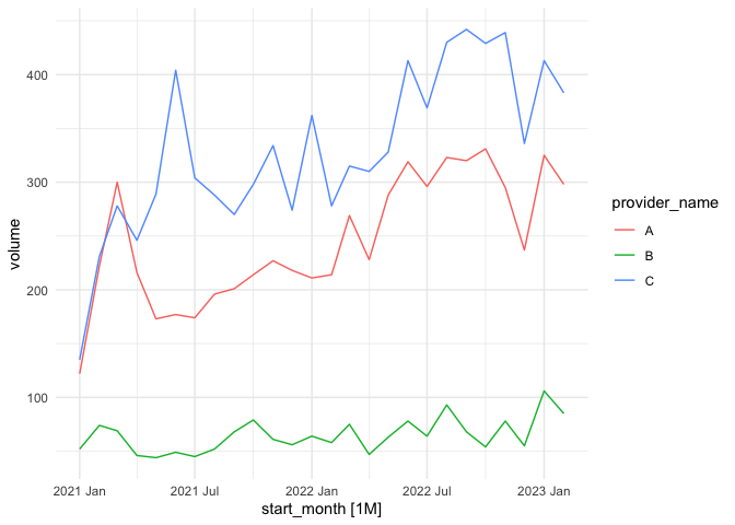
Here's a worked example using your data with some of the tools described in the Hyndman text. It's a useful template, beginning with an initial visualization, look at how the three provider series differ, and for one of them, A, some more detailed work, including a comparison of years, a look at autocorrelation, decomposition into seasonal, trend and residual components, division into training and test sets, development of baseline models, a forecast, evaluation and diagnostics. Then one of the many more advanced models, ARIMA, is selected to see if it can do better.
Going through the text following the example with your own data will help understand all the pieces, and if you get stuck, come back in a new thread with a reprex like I've used and questions.
Despite the equations, the core of forecasting is that the future looks like the past (until it doesn't, because something in the processes that created the historical data has changed).
library(fpp3)
#> ── Attaching packages ────────────────────────────────────────────── fpp3 0.5 ──
#> ✔ tibble      3.2.1     ✔ tsibble     1.1.3
#> ✔ dplyr       1.1.1     ✔ tsibbledata 0.4.1
#> ✔ tidyr       1.3.0     ✔ feasts      0.3.1
#> ✔ lubridate   1.9.2     ✔ fable       0.3.3
#> ✔ ggplot2     3.4.1     ✔ fabletools  0.3.2
#> ── Conflicts ───────────────────────────────────────────────── fpp3_conflicts ──
#> ✖ lubridate::date()    masks base::date()
#> ✖ dplyr::filter()      masks stats::filter()
#> ✖ tsibble::intersect() masks base::intersect()
#> ✖ tsibble::interval()  masks lubridate::interval()
#> ✖ dplyr::lag()         masks stats::lag()
#> ✖ tsibble::setdiff()   masks base::setdiff()
#> ✖ tsibble::union()     masks base::union()

s_data <- structure(list(
  provider_name = c(
    "A", "A", "A", "A", "A", "A",
    "A", "A", "A", "A", "A", "A", "A", "A", "A", "A", "A", "A", "A",
    "A", "A", "A", "A", "A", "A", "A", "B", "B", "B", "B", "B", "B",
    "B", "B", "B", "B", "B", "B", "B", "B", "B", "B", "B", "B", "B",
    "B", "B", "B", "B", "B", "B", "B", "C", "C", "C", "C", "C", "C",
    "C", "C", "C", "C", "C", "C", "C", "C", "C", "C", "C", "C", "C",
    "C", "C", "C", "C", "C", "C", "C"
  ), start_month = c(
    "2021 Jan",
    "2021 Feb", "2021 Mar", "2021 Apr", "2021 May", "2021 Jun", "2021 Jul",
    "2021 Aug", "2021 Sep", "2021 Oct", "2021 Nov", "2021 Dec", "2022 Jan",
    "2022 Feb", "2022 Mar", "2022 Apr", "2022 May", "2022 Jun", "2022 Jul",
    "2022 Aug", "2022 Sep", "2022 Oct", "2022 Nov", "2022 Dec", "2023 Jan",
    "2023 Feb", "2021 Jan", "2021 Feb", "2021 Mar", "2021 Apr", "2021 May",
    "2021 Jun", "2021 Jul", "2021 Aug", "2021 Sep", "2021 Oct", "2021 Nov",
    "2021 Dec", "2022 Jan", "2022 Feb", "2022 Mar", "2022 Apr", "2022 May",
    "2022 Jun", "2022 Jul", "2022 Aug", "2022 Sep", "2022 Oct", "2022 Nov",
    "2022 Dec", "2023 Jan", "2023 Feb", "2021 Jan", "2021 Feb", "2021 Mar",
    "2021 Apr", "2021 May", "2021 Jun", "2021 Jul", "2021 Aug", "2021 Sep",
    "2021 Oct", "2021 Nov", "2021 Dec", "2022 Jan", "2022 Feb", "2022 Mar",
    "2022 Apr", "2022 May", "2022 Jun", "2022 Jul", "2022 Aug", "2022 Sep",
    "2022 Oct", "2022 Nov", "2022 Dec", "2023 Jan", "2023 Feb"
  ),
  volume = c(
    122L, 222L, 300L, 216L, 173L, 177L, 174L, 196L,
    201L, 214L, 227L, 218L, 211L, 214L, 269L, 228L, 288L, 319L,
    296L, 323L, 320L, 331L, 295L, 237L, 325L, 298L, 52L, 74L,
    69L, 46L, 44L, 49L, 45L, 52L, 68L, 79L, 61L, 56L, 64L, 58L,
    75L, 47L, 63L, 78L, 64L, 93L, 68L, 54L, 78L, 55L, 106L, 85L,
    135L, 231L, 278L, 246L, 289L, 404L, 304L, 288L, 270L, 298L,
    334L, 274L, 362L, 278L, 315L, 310L, 328L, 413L, 369L, 430L,
    442L, 429L, 439L, 336L, 413L, 383L
  )
), class = c(
  "tbl_df",
  "tbl", "data.frame"
), row.names = c(NA, -78L))

ts_data <- s_data %>%
  mutate(start_month = tsibble::yearmonth(start_month)) %>%
  as_tsibble(index = start_month,
             key = provider_name)

# first step is always to eyeball the data
autoplot(ts_data) + theme_minimal()
#> Plot variable not specified, automatically selected `.vars = volume`
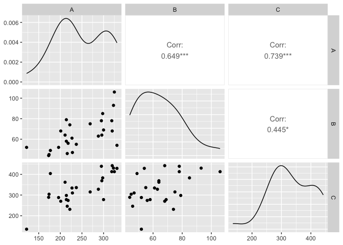
ts_data |>
  pivot_wider(values_from=volume, names_from=provider_name) |>
  GGally::ggpairs(columns = 2:4)
#> Registered S3 method overwritten by 'GGally':
#>   method from
#>   +.gg   ggplot2
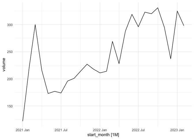
# pick provider A to begin

tsA <- ts_data %>% filter(provider_name == "A")
tsA$month_no <- 1:26

autoplot(tsA) + theme_minimal()
#> Plot variable not specified, automatically selected `.vars = volume`
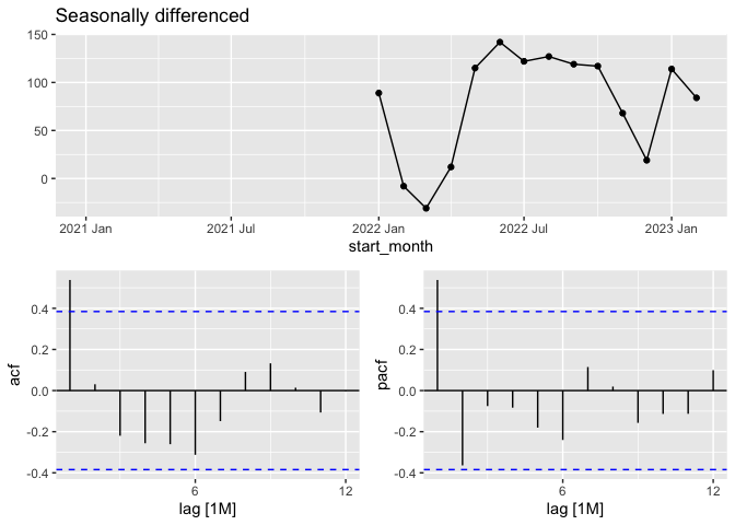
tsA |>
  gg_tsdisplay(difference(volume, 12),
               plot_type='partial', lag=12) +
  labs(title="Seasonally differenced", y="")
#> Warning: Removed 12 rows containing missing values (`geom_line()`).
#> Warning: Removed 12 rows containing missing values (`geom_point()`).
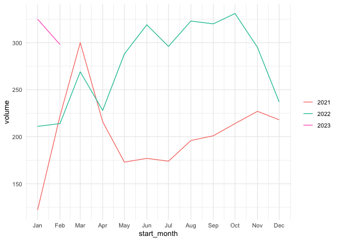
# comparison of years
tsA %>% gg_season(volume) + theme_minimal()
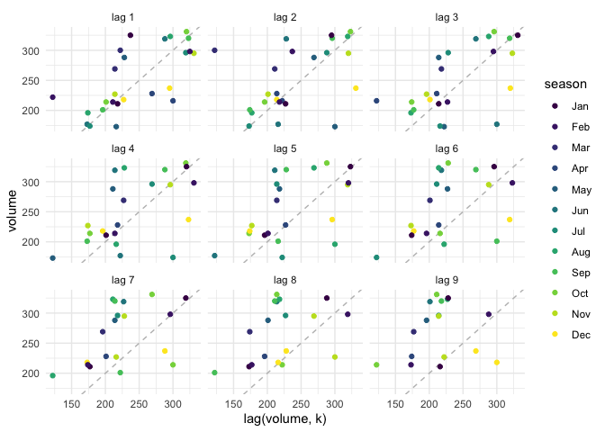
# lags
tsA |> gg_lag(volume, geom = "point") +
  labs(x = "lag(volume, k)") +
  theme_minimal()
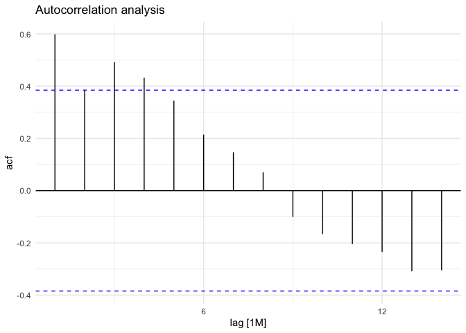
# autocorrelation
tsA %>%
  ACF(volume) %>%
  autoplot() + labs(title="Autocorrelation analysis") +
  theme_minimal()
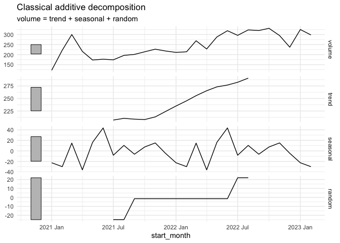
# decomposition

tsA |>
  model(
    classical_decomposition(volume, type = "additive")
  ) |>
  components() |>
  autoplot() +
  labs(title = "Classical additive decomposition") +
  theme_minimal()
#> Warning: Removed 6 rows containing missing values (`geom_line()`).
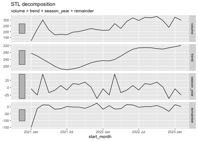
# STL decomposition

tsA |>
  model(
    STL(volume ~ trend(window = 7) +
          season(window = "periodic"),
        robust = TRUE)) |>
  components() |>
  autoplot() ;+
  theme_minimal()
#> Error in `e1 %+% e2`:
#> ! Cannot use `+` with a single argument
#> ℹ Did you accidentally put `+` on a new line?
#> Backtrace:
#>     ▆
#>  1. └─GGally:::`+.gg`(theme_minimal())
#>  2.   └─e1 %+% e2
#>  3.     └─cli::cli_abort(...)
#>  4.       └─rlang::abort(...)
# example features summary
tsA |> features(volume, quantile)
#> # A tibble: 1 × 6
#> provider_name `0%` `25%` `50%` `75%` `100%`
#> <chr> <dbl> <dbl> <dbl> <dbl> <dbl>
#> 1 A 122 212. 228. 298. 331
# baseline models
# Set training data from 2021 Jan to 2022 Oct
train <- tsA|> filter_index("2021 Jan" ~ "2022 Oct")
# test data from 2022 Nov to 2023 Feb
test <- tsA|> filter_index("2022 Nov" ~ "2023 Feb")
# Fit the models
fit <- train |>
model(
Mean = MEAN(volume),
`Naïve` = NAIVE(volume),
`Seasonal naïve` = SNAIVE(volume)
)
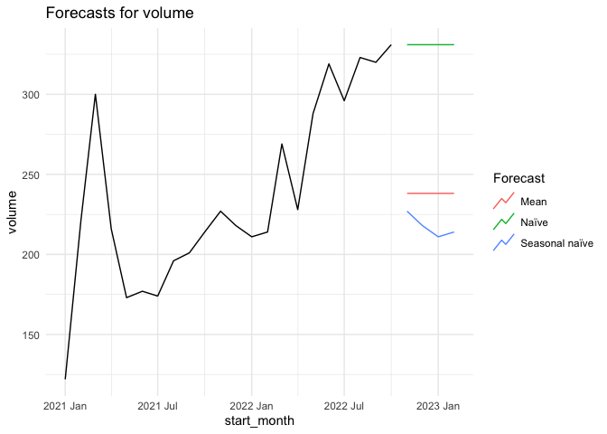
# Generate forecasts for 4 months
fc <- fit |> forecast(h = 4)
# Plot forecasts against actual values
fc |>
autoplot(train, level = NULL) +
autolayer(
filter_index(tsA, "2023 Feb" ~ .),
colour = "black"
) +
labs(
y = "volume",
title = "Forecasts for volume"
) +
guides(colour = guide_legend(title = "Forecast")) +
theme_minimal()
#> Plot variable not specified, automatically selected `.vars = volume`
#> `geom_line()`: Each group consists of only one observation.
#> ℹ Do you need to adjust the group aesthetic?
augment(fit)
#> # A tsibble: 66 x 7 [1M]
#> # Key: provider_name, .model [3]
#> provider_name .model start_month volume .fitted .resid .innov
#> <chr> <chr> <mth> <int> <dbl> <dbl> <dbl>
#> 1 A Mean 2021 Jan 122 238. -116. -116.
#> 2 A Mean 2021 Feb 222 238. -16.1 -16.1
#> 3 A Mean 2021 Mar 300 238. 61.9 61.9
#> 4 A Mean 2021 Apr 216 238. -22.1 -22.1
#> 5 A Mean 2021 May 173 238. -65.1 -65.1
#> 6 A Mean 2021 Jun 177 238. -61.1 -61.1
#> 7 A Mean 2021 Jul 174 238. -64.1 -64.1
#> 8 A Mean 2021 Aug 196 238. -42.1 -42.1
#> 9 A Mean 2021 Sep 201 238. -37.1 -37.1
#> 10 A Mean 2021 Oct 214 238. -24.1 -24.1
#> # ℹ 56 more rows
# the naive model tests best on more measures
accuracy(fc, test)[c(1,4:8)]
#> # A tibble: 3 × 6
#> .model ME RMSE MAE MPE MAPE
#> <chr> <dbl> <dbl> <dbl> <dbl> <dbl>
#> 1 Mean 50.6 59.9 51.2 16.4 16.6
#> 2 Naïve -42.2 53.0 42.2 -16.2 16.2
#> 3 Seasonal naïve 71.2 79.1 71.2 23.6 23.6
fit <- train |> model(naif = NAIVE(volume))
report(fit)
#> Series: volume
#> Model: NAIVE
#>
#> sigma^2: 1728.7476
# fit some ARIMA models
fit <- tsA |>
model(arima210 = ARIMA(volume ~ pdq(2,1,0)),
arima013 = ARIMA(volume ~ pdq(0,1,3)),
stepwise = ARIMA(volume),
search = ARIMA(volume, stepwise=FALSE))
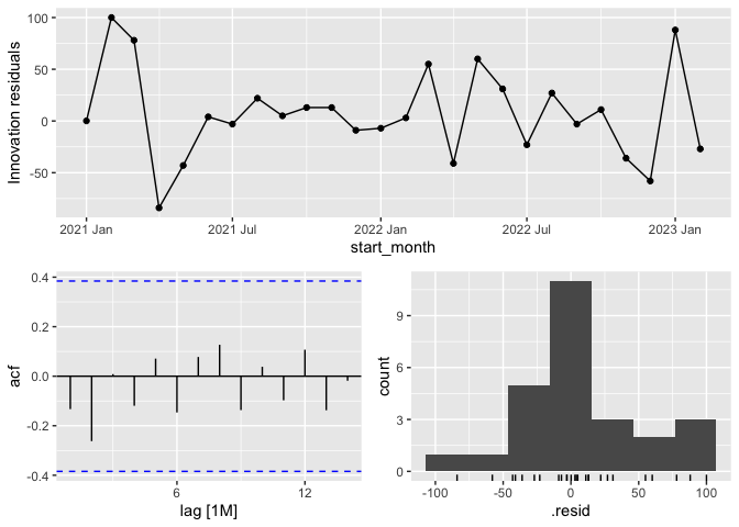
# diagnostics
glance(fit) |> arrange(AICc) |> select(.model:BIC)
#> # A tibble: 4 × 6
#> .model sigma2 log_lik AIC AICc BIC
#> <chr> <dbl> <dbl> <dbl> <dbl> <dbl>
#> 1 stepwise 1992. -130. 263. 263. 264.
#> 2 search 1992. -130. 263. 263. 264.
#> 3 arima210 1771. -128. 263. 264. 266.
#> 4 arima013 1758. -128. 263. 265. 268.
fit |>
select(search) |>
gg_tsresiduals()
augment(fit) |>
filter(.model=='search') |>
features(.innov, ljung_box, lag = 10, dof = 3)
#> # A tibble: 1 × 4
#> provider_name .model lb_stat lb_pvalue
#> <chr> <chr> <dbl> <dbl>
#> 1 A search 5.78 0.566
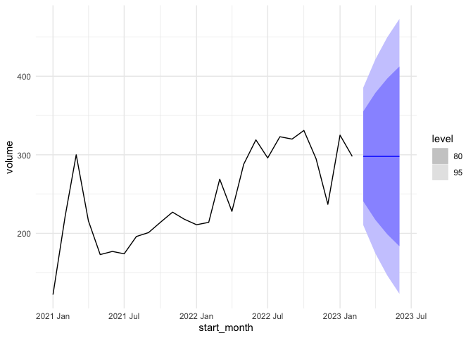
fit |>
forecast(h=4) |>
filter(.model=='search') |>
autoplot(tsA) +
theme_minimal()
Created on 2023-04-03 with reprex v2.0.2
This topic was automatically closed 21 days after the last reply. New replies are no longer allowed.
If you have a query related to it or one of the replies, start a new topic and refer back with a link.