Here's a listing of all the code up to the failure point. I have added dputs at different points in the code. I hope that helps. This run is with a csv file with a number of lines that executes correctly.
#start====
library(tidyverse)
library(readxl)
library(readr)
library(lubridate)
library(hms)
library(nortest)
library("viridis")
setwd("C:\\Users\\tom_s\\OneDrive\\Documents\\Solar Energy Project")
getwd()
source("Tukey_Plot_Function.R")
source("Useful Functions.R")
# DATA IMPORT====
#Set up year for analysis
# Choose a year in the range 2020-2025 or 1 for analysis of all years data
analyse_year<-2025
# Import Raw Data====
# Import the raw data from downloaded Brusol data. Select only columns 1 and 5.
# The function read_csv2 uses semi-colons as the separator and stores the data in a variable called raw_data
raw_Measures <- read_csv2("measures_solar_all.csv",col_select = c(1,5),show_col_types = FALSE)
# we can test to see of there are any errors (na) in the imported data. We find these using the following instruction
which(is.na(raw_Measures$timestamp), arr.ind=TRUE)
# In this case there are two at 5996 and 13980
# We can check the source of the nas (they are on month boundaries and are, in fact, user error!
# They are both copy and paste errors made while aggregrating monthly data)
raw_Measures[c(5995:5997,13979:13981),]
dput(raw_Measures[108995:109005, ])
# Rather than read in data each time from a csv, we can create an rds object and then read that in for the analysis.
write_rds(raw_Measures,"all_raw_measures.rds")
# In future we use the data in the rds object
rm(raw_Measures)
# We can read in the rds object as follows. using the same variable (dataframe)
# name means we can use all the following code without modification
# First, I rename value to WattHour, a useful name in the context
# Omit the "known" errors used to illustrate how to find nas in the input file
raw_Measures <- read_rds("all_raw_measures.rds")%>% rename(WattHour = value)%>%na.omit()
summary(raw_Measures$WattHour)
energy_raw_1=sum(raw_Measures$WattHour)
dput(raw_Measures[108995:109005, ])
# We need now to remove the zeros that occur before sunrise and after sunset
# (while accounting for occlusion in the built environment!)
dput(raw_Measures[108995:109005, ])
# We are now able to extract information for use in the grouping and plotting of data for the analysis and charts.
# In this section I use a number of functions from the lubridate library.
# The plots are prepared using the ggplot library in tidyverse.
# The variable called processed_measures will hold the modified data for subsequent editing.
#Processed Data====
# Add a sunshine ID (SID) to allow easy joining of datasets or filtering by joins
#Extract variety of data from the timestamp using lubridate and pass the data to a new variable called processed_Measures
processed_Measures<-raw_Measures%>%
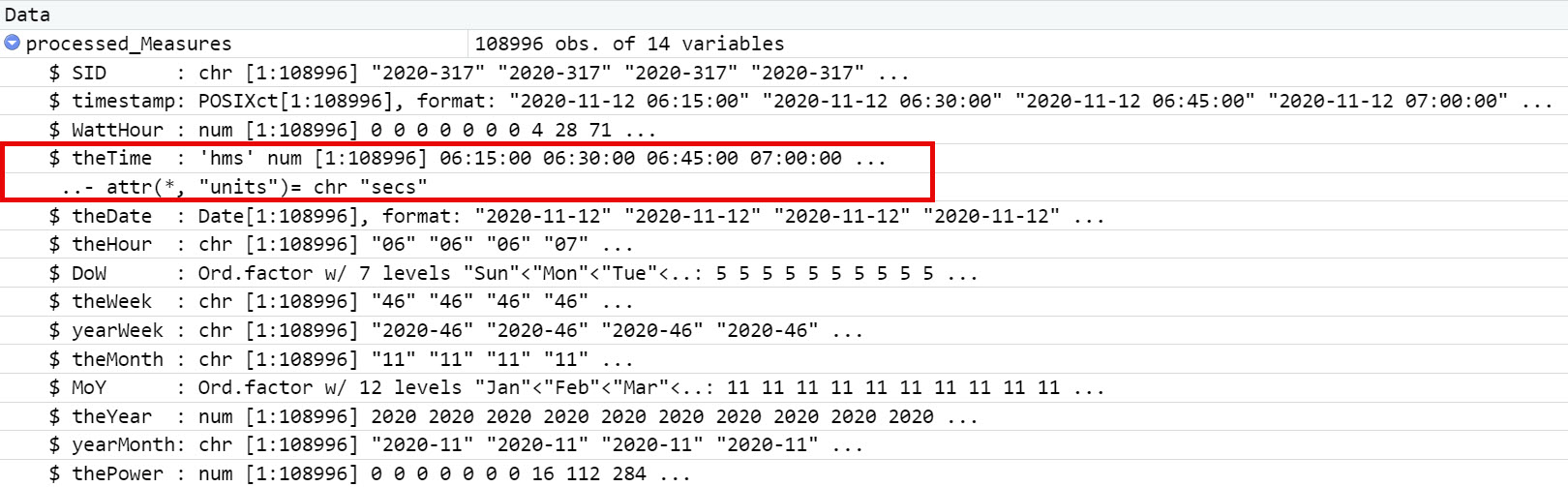
mutate(SID=paste0(as.character(year(timestamp)),"-",sprintf("%03d",yday(timestamp))),theTime=as_hms(timestamp),
theDate=date(timestamp),
theHour=sprintf("%02d",hour(timestamp)),
DoW=wday(timestamp, label = TRUE),
theWeek=sprintf("%02d",week(timestamp)),
yearWeek=paste0(as.character(year(timestamp)),"-",sprintf("%02d",week(timestamp))),
theMonth=sprintf("%02d",month(timestamp)),
MoY=month(timestamp, label = TRUE),
theYear=year(timestamp),
yearMonth=paste0(as.character(year(timestamp)),"-",sprintf("%02d",month(timestamp))),
thePower=4*WattHour
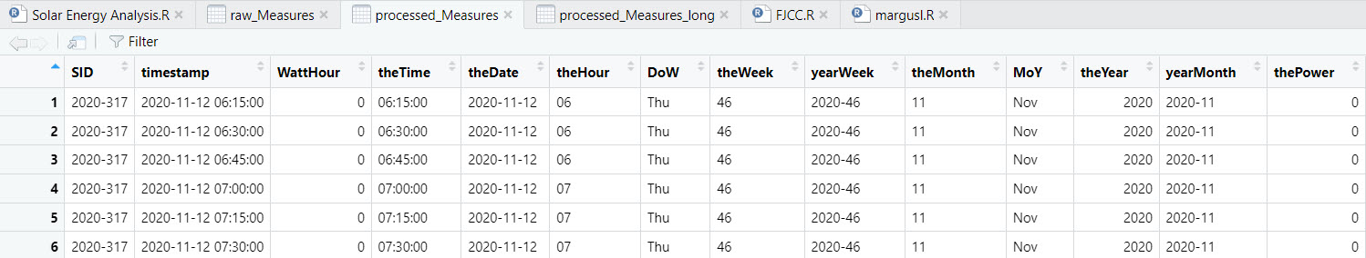
)%>%relocate(SID)
The output screen looks like this:
#start====
> library(tidyverse)
> library(readxl)
> library(readr)
> library(lubridate)
> library(hms)
> library(nortest)
> library("viridis")
>
> setwd("C:\\Users\\tom_s\\OneDrive\\Documents\\Solar Energy Project")
> getwd()
[1] "C:/Users/tom_s/OneDrive/Documents/Solar Energy Project"
> source("Tukey_Plot_Function.R")
> source("Useful Functions.R")
> # DATA IMPORT====
> #Set up year for analysis
> # Choose a year in the range 2020-2025 or 1 for analysis of all years data
> analyse_year<-2025
>
> # Import Raw Data====
> # Import the raw data from downloaded Brusol data. Select only columns 1 and 5.
> # The function read_csv2 uses semi-colons as the separator and stores the data in a variable called raw_data
>
> raw_Measures <- read_csv2("measures_solar_all.csv",col_select = c(1,5),show_col_types = FALSE)
ℹ Using "','" as decimal and "'.'" as grouping mark. Use `read_delim()` for more control.
Warning message:
One or more parsing issues, call `problems()` on your data frame for details, e.g.:
  dat <- vroom(...)
  problems(dat)
>
> # we can test to see of there are any errors (na) in the imported data. We find these using the following instruction
> which(is.na(raw_Measures$timestamp), arr.ind=TRUE)
[1]   5996  13980 106620
> # In this case there are two at 5996 and 13980
> # We can check the source of the nas (they are on month boundaries and are, in fact, user error!
> # They are both copy and paste errors made while aggregrating monthly data)
> raw_Measures[c(5995:5997,13979:13981),]
# A tibble: 6 × 2
  timestamp           value
  <dttm>              <dbl>
1 2021-02-28 19:45:00     0
2 NA                      0
3 2021-03-01 06:30:00     0
4 2021-06-30 22:30:00     0
5 NA                      0
6 2021-07-01 05:45:00     0
> dput(raw_Measures[108995:109005, ])
structure(list(timestamp = structure(c(1753723800, 1753724700,
1753725600, 1753726500, 1753727400, NA, NA, NA, NA, NA, NA), tzone = "UTC", class = c("POSIXct",
"POSIXt")), value = c(176, 139, 103, 85, 61, NA, NA, NA, NA,
NA, NA)), row.names = c(NA, -11L), class = c("tbl_df", "tbl",
"data.frame"), spec = structure(list(cols = list(timestamp = structure(list(
    format = ""), class = c("collector_datetime", "collector"
)), meter.identification = structure(list(), class = c("collector_skip",
"collector")), meter.name = structure(list(), class = c("collector_skip",
"collector")), meter.type = structure(list(), class = c("collector_skip",
"collector")), value = structure(list(), class = c("collector_double",
"collector")), meter.unit = structure(list(), class = c("collector_skip",
"collector"))), default = structure(list(), class = c("collector_guess",
"collector")), delim = ";"), class = "col_spec"))
> # Rather than read in data each time from a csv, we can create an rds object and then read that in for the analysis.
> write_rds(raw_Measures,"all_raw_measures.rds")
> # In future we use the data in the rds object
> rm(raw_Measures)
>
> # We can read in the rds object as follows. using the same variable (dataframe)
> # name means we can use all the following code without modification
> # First, I rename value to WattHour, a useful name in the context
> # Omit the "known" errors used to illustrate how to find nas in the input file
> raw_Measures <- read_rds("all_raw_measures.rds")%>% rename(WattHour = value)%>%na.omit()
> summary(raw_Measures$WattHour)
   Min. 1st Qu.  Median    Mean 3rd Qu.    Max.
    0.0     0.0    52.0   167.4   258.0   916.0
> energy_raw_1=sum(raw_Measures$WattHour)
> dput(raw_Measures[108995:109005, ])
structure(list(timestamp = structure(c(1753726500, 1753727400,
NA, NA, NA, NA, NA, NA, NA, NA, NA), tzone = "UTC", class = c("POSIXct",
"POSIXt")), WattHour = c(85, 61, NA, NA, NA, NA, NA, NA, NA,
NA, NA)), row.names = c(NA, -11L), class = c("tbl_df", "tbl",
"data.frame"), spec = structure(list(cols = list(timestamp = structure(list(
    format = ""), class = c("collector_datetime", "collector"
)), meter.identification = structure(list(), class = c("collector_skip",
"collector")), meter.name = structure(list(), class = c("collector_skip",
"collector")), meter.type = structure(list(), class = c("collector_skip",
"collector")), value = structure(list(), class = c("collector_double",
"collector")), meter.unit = structure(list(), class = c("collector_skip",
"collector"))), default = structure(list(), class = c("collector_guess",
"collector")), delim = ";"), class = "col_spec"), na.action = structure(c(`5996` = 5996L,
`13980` = 13980L, `106620` = 106620L), class = "omit"))
> # We need now to remove the zeros that occur before sunrise and after sunset
> # (while accounting for occlusion in the built environment!)
>
> # Import sunrise/sunset data from https://robinfo.oma.be/en/astro-info/sun/sunrise-sunset-2025/
> # The Royal Observatory of Belgium
> # This is currently in the Excel file in the working directory where the data have been wrangled into shape.
> # This will let us filter out fixed-time zeros in the data to ensure accurate and meaningful data analysis
>
> dput(raw_Measures[108995:109005, ])
structure(list(timestamp = structure(c(1753726500, 1753727400,
NA, NA, NA, NA, NA, NA, NA, NA, NA), tzone = "UTC", class = c("POSIXct",
"POSIXt")), WattHour = c(85, 61, NA, NA, NA, NA, NA, NA, NA,
NA, NA)), row.names = c(NA, -11L), class = c("tbl_df", "tbl",
"data.frame"), spec = structure(list(cols = list(timestamp = structure(list(
    format = ""), class = c("collector_datetime", "collector"
)), meter.identification = structure(list(), class = c("collector_skip",
"collector")), meter.name = structure(list(), class = c("collector_skip",
"collector")), meter.type = structure(list(), class = c("collector_skip",
"collector")), value = structure(list(), class = c("collector_double",
"collector")), meter.unit = structure(list(), class = c("collector_skip",
"collector"))), default = structure(list(), class = c("collector_guess",
"collector")), delim = ";"), class = "col_spec"), na.action = structure(c(`5996` = 5996L,
`13980` = 13980L, `106620` = 106620L), class = "omit"))
> # We are now able to extract information for use in the grouping and plotting of data for the analysis and charts.
> # In this section I use a number of functions from the lubridate library.
> # The plots are prepared using the ggplot library in tidyverse.
> # The variable called processed_measures will hold the modified data for subsequent editing.
>
> #Processed Data====
> # Add a sunshine ID (SID) to allow easy joining of datasets or filtering by joins
> #Extract variety of data from the timestamp using lubridate and pass the data to a new variable called processed_Measures
> processed_Measures<-raw_Measures%>%
+    mutate(SID=paste0(as.character(year(timestamp)),"-",sprintf("%03d",yday(timestamp))),theTime=as_hms(timestamp),
+    theDate=date(timestamp),
+    theHour=sprintf("%02d",hour(timestamp)),
+    DoW=wday(timestamp, label = TRUE),
+    theWeek=sprintf("%02d",week(timestamp)),
+    yearWeek=paste0(as.character(year(timestamp)),"-",sprintf("%02d",week(timestamp))),
+    theMonth=sprintf("%02d",month(timestamp)),
+    MoY=month(timestamp, label = TRUE),
+    theYear=year(timestamp),
+    yearMonth=paste0(as.character(year(timestamp)),"-",sprintf("%02d",month(timestamp))),
+    thePower=4*WattHour
+    )%>%relocate(SID)
>
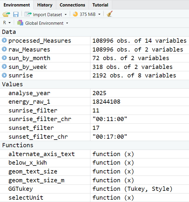
The global environment shows the successful processing of data. When I add a single extra, correctly-formatted row to the csv file the code stops.