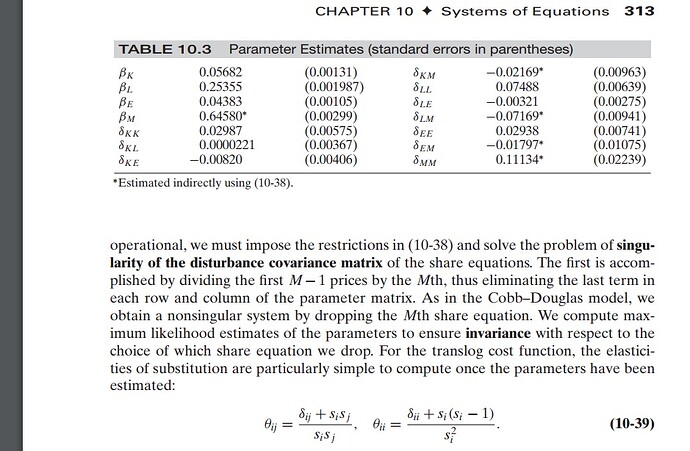
Howdy. Other than the setup, this isn't really an R or RStudio question. But happy to help. It's been 8 years for me spending much time with Greene
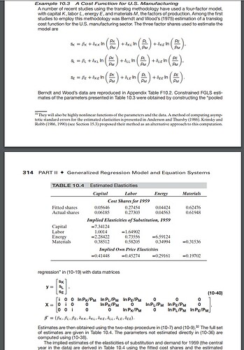
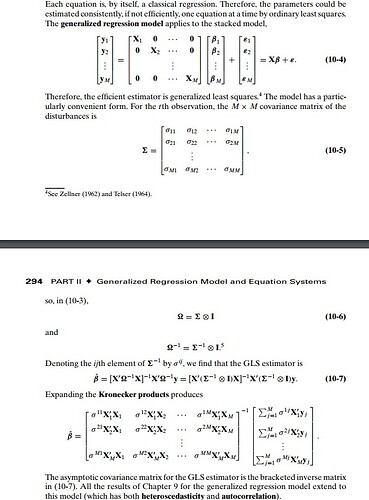
The model setup by eq 10-40 is, I think:
costdata = read.csv(".../TableF10-2.csv")

# setup dependent vars for /delta_...
costdata = costdata %>%
  mutate(
    lnpkpm = log(Pk / Pm),
    lnplpm = log(Pl / Pm),
    lnpepm = log(Pe / Pm)
    )
setup eq 10-40:
df_pooledreg <-
  bind_rows(
    tibble(
      y = costdata$K,
      k = 1,
      l = 0,
      e = 0,
      kk = costdata$lnpkpm,
      kl = costdata$lnplpm,
      ke = costdata$lnpepm,
      ll = 0,
      le = 0,
      ee = 0,
      year = costdata$Year
    ),
    tibble(
      y = costdata$L,
      k = 0,
      l = 1,
      e = 0,
      kk = 0,
      kl = costdata$lnpkpm,
      ke = 0,
      ll = costdata$lnplpm,
      le = costdata$lnpepm,
      ee = 0,
      year = costdata$Year
    ),
    tibble(
      y = costdata$E,
      k = 0,
      l = 0,
      e = 1,
      kk = 0,
      kl = 0,
      ke = costdata$lnpkpm,
      ll = 0,
      le = costdata$lnplpm,
      ee = costdata$lnpepm,
      year = costdata$Year
    )
  )
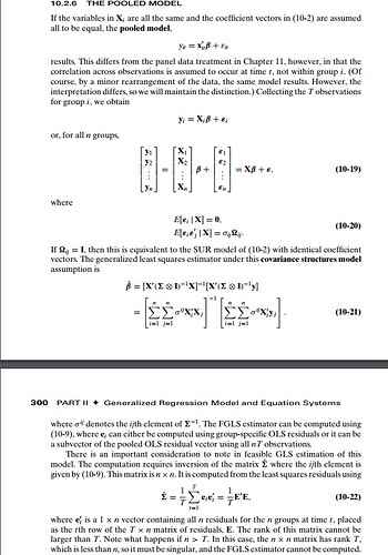
run "The Pooled Model" eq 10-19 in Greene chapter 10.
Note, eq 10-19 doesn't have an intercept.
pooledreg = glm(
  y ~ 0 + k + l + e + kk + kl + ke + ll +le + ee,
  data = df_pooledreg
)
summary(pooledreg)
I get the following coefficients:
Coefficients:
    Estimate Std. Error t value Pr(>|t|)
k   0.056223   0.001888  29.773  < 2e-16 ***
l   0.253409   0.001852 136.834  < 2e-16 ***
e   0.041861   0.002291  18.272  < 2e-16 ***
kk  0.030426   0.008067   3.772 0.000349 ***
kl  0.001755   0.004556   0.385 0.701342
ke -0.003562   0.007481  -0.476 0.635562
ll  0.075127   0.005280  14.228  < 2e-16 ***
le  0.003252   0.005756   0.565 0.574043
ee  0.046777   0.017415   2.686 0.009136 **
---
Now, Table 10.4. The first line, Fitted shares is just:
fitted_k = predict(
  pooledreg,
  df_pooledreg %>% filter(year == 1959 & k)
)
fitted_l = predict(
  pooledreg,
  df_pooledreg %>% filter(year == 1959 & l)
)
fitted_e = predict(
  pooledreg,
  df_pooledreg %>% filter(year == 1959 & e)
)
# Note that assuming a constant returns to scale production function,
# `m` is just `1-(k+l+e) `
fitted_m = 1 - (fitted_k + fitted_l + fitted_e)
fitted_k: 0.05655583
fitted_l: 0.2747627
fitted_e: 0.04487152
fitted_m: 0.6238099
How do we estimate the derivatives involving Materials? i.e. those $/delta_{M...}$? For that, turn to equation 10-38 (well, it's eq 10-38 in my Greene, 6th edition of econometric analysis anyway. they seem to be moving things around). That equation just says,
$\Sigma_{i=1}^M \delta_{ij} = 0$ and $\Sigma_{j=1}^M \delta_{ij} = 0$.
Really simple, you can see this in table 10.4. It just says that $\delta_{KK} + $\delta_{KL} + $\delta_{KE} + $\delta_{KM} = 0.
You'll notice in table 10.4 any derivative with an M has an asterisks next to it, referring to eq 10-38.
Equation 10-39 gives the own and cross elasticities of substitution.
So with $\theta_{kk}$ for example, (/delta_{kk} + s_{i}(s_{i} - 1)) / s_{i}^2, where i is capital share's output in that year.
or with my estimates and your data:
s_k1959 = ((costdata %>% filter(Year == 1959)))$K
delta_kk = pooledreg$coefficients['kk'] %>% as.vector
(delta_kk + s_k1959 * (s_k1959 - 1)) / (s_k1959^2)
[1] -7.214395 # that's under "Implied Elasticities of Substitution, 1959" for Capital/Capital
And for cross price elasticity of substitution, eq 10-39 says
$\theta_{ij}$ is , (/delta_{ij} + s_{i} * s{j}) / (s_{i} * s_{j}),
for example for $\theta_{KL}$:
s_k1959 = ((costdata %>% filter(Year == 1959)))$K
s_l1959 = ((costdata %>% filter(Year == 1959)))$L
delta_kl = pooledreg$coefficients['kl'] %>% as.vector
(delta_kl + (s_k1959 * s_l1959)) / (s_k1959 * s_l1959)
[1] 1.103912 # this is our estimate for "Implied Elasticities of Substitution, 1959" for Labor/Capital
There are slight deviations. They might come from using an updated dataset...?
