See blog on adding manual legend as well as this RStudio community post Adding manual legend to ggplot2 to add in custom legends when aes() aren't called. Personal preference the first link is less hacky than the second. As legend title and legend text should be adjusted using names and labels arguments in scale_colour_manual(). For your situation you'll have to move colour = "red" into aes(). Then manual change both the colour and label with something like scale_colour_manual()
@benjaminhlina Thanks for your suggestion. I do have some applications that where I would have to make a bunch of smaller data frames!
thanks again!
@benjaminhlina Thanks again for your suggestion. I would like to use your method, however, I am running into some errors.
The first reprex is the code that is working and used geometric mean values from another data frame ("GeomMean2")
graph3 <- ocoee %>%
  filter(parm =="tn", year>2009) %>%
  ggplot() +
  geom_point(mapping =aes(x=date, y=value, color=source)) +
  geom_point(mapping = aes(MyDate2, GMean2), data = GeomMean2, size = 1, color = "red") +
  geom_line(mapping = aes(MyDate2, GMean2, linetype=GeoMean), data = GeomMean2, size = 1, color = "purple") +
  scale_x_date(date_breaks = "1 years", date_labels = "%Y") +
  labs(x="Year", y="TN (mg/L)")+
  theme(legend.position = "bottom") +
  facet_wrap(~lake, ncol=1, scales= "free", labeller = labeller(lake=lak.labs))
#> Error in ocoee %>% filter(parm == "tn", year > 2009) %>% ggplot(): could not find function "%>%"
graph3
#> Error in eval(expr, envir, enclos): object 'graph3' not found
Created on 2020-11-20 by the reprex package (v0.3.0)
The second code uses your suggestion--I clearly did something wrong. And again, I am trying to plot a scatterplot and a line with points representing geometric mean values for each year. (I am also getting a reprex error when I try to reprex this selection--I tried to trouble shoot this, but could not figure this out!?)
graph3 <- ocoee %>%
filter(parm =="tn", year>2009) %>%
ggplot() +
geom_point(mapping =aes(x=date, y=value, color=source)) +
geom = "point", fun = exp(mean(log(value))) +
geom = "line" fun = exp(mean(log(value))) +
scale_x_date(date_breaks = "1 years", date_labels = "%Y") +
labs(x="Year", y="TN (mg/L)")+
theme(legend.position = "bottom") +
scale_color_manual()
facet_wrap(~lake, ncol=1, scales= "free", labeller = labeller(lake=lak.labs))
graph3
You need to use the function stat_summary() see link to ggplot2 reference. I'm unsure if stat_summary() can handle a function expression like that. I've used it several times just to determine the mean and figured it would probably work to calculate what you need...it may not but regardless you need to use the function stat_summary(). You then need to look at what arguments are needed which what you have currently in your code. Side note, the use of the mapping argument is redundant, you can just use aes(). The only time you need to call mapping is if you're doing some more complex plots than what you are using it for.
The reason why the first is erroring is you need to load either dplyr or magrittr as they have the pipe function %>%.
This is also a stylistic thing, space after every operator and comma i.e. x = date ect. Set a margin in gobal options of 80 characters as it keeps the code from trailing off. Notice how I've entered and tabbed everything and things are in a left to right top to bottom order. This is much easier to read and write than code that continues to trail off forever.
Notice also how I've changed the order in which facet_wrap(), scale_x_date(), theme(), and labs() are being called...this reads much easier as you start the plot with the data you want plotted, you then move to making multiple plots with facet_wrap(), change the axis, then change the underlying themes, and lastly finish with labels.
You'll also notice that I changed your code for the label to mg L^-1 which will result in a subscript of -1 and looks way better than mg/l
graph3 <- ocoee %>%
  filter(parm == "tn", year > 2009) %>%
  ggplot() +
  geom_point(aes(x = date, y = value, color = source)) +
  geom_point(data = GeomMean2,
             aes(x = MyDate2, y = GMean2),
             size = 1,
             color = "red") +
  geom_line(data = GeomMean2,
            aes(x = MyDate2, y = GMean2, linetype = GeoMean),
            size = 1,
            color = "purple") +
  facet_wrap(.~ lake, ncol = 1, scales =  "free",
             labeller = labeller(lake = lak.labs))
  scale_x_date(date_breaks = "1 years", date_labels = "%Y") +
  theme(legend.position = "bottom") +
  labs(x = "Year", y = expression(paste("TN (mg ", L^-1), ")")))
You can use this little function and then use stat_summary(). See this stackoverflow link....I simply googled the following "how to use stat_summary in for geometric mean" and the second link has an answer.
gm_mean <- function(x) {
 exp(mean(log(x)))
}

graph3 <- ocoee %>%
  filter(parm == "tn", year > 2009) %>%
  ggplot() +
  geom_point(aes(x = date, y = value, color = source)) +
  stat_summary(aes(x = date, y = value), fun = gm_mean,
               geom = "point",
               size = 1,
               color = "red") +
  stat_summary(aes(x = date, y = value, linetype = source),
               fun = gm_mean,
               geom = "line"
               size = 1,
               color = "purple") +
  facet_wrap(.~ lake, ncol = 1, scales =  "free",
             labeller = labeller(lake = lak.labs))
  scale_x_date(date_breaks = "1 years", date_labels = "%Y") +
  theme(legend.position = "bottom") +
  labs(x = "Year", y = expression(paste("TN (mg ", L^-1), ")")))
@benjaminhlina---thanks for these stylistic reccomendations--especially the spaces. Much easier to read.
Also, thanks for the facet_wrap order changes--I have wondered about this, and never seen a clear answer.
Finally, yes on the mg/L--way better
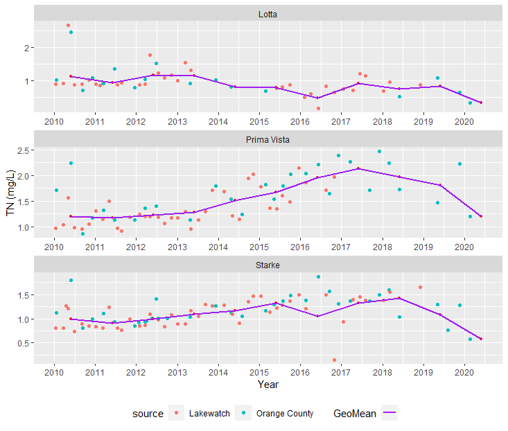
@benjaminhlina This code certainly simplifies thing, however, I am actually looking for the annual geometric means (i.e., geo mean of all values in 2010, 2011, etc.). The code looks like it is producing the geometric mean for that specific date? I looked at the stackoverflow page that you cited, and could not see anything about specifying a certain group for geo mean calcuation.
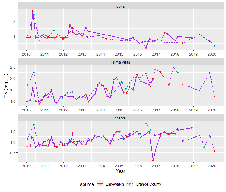
This is the plot that was created:
As far as the stylistic changes/order in which you call functions in ggplot. You can call ggplot functions however you want under ggplot() + but the idea that Hadley has around ggplot is that you build a figure in layers that follow a logical order hence the order that I provided which is the order Hadley uses in his books/documentation of ggplot.
The SO link I provided gives you the geometic mean function..this is where knowing a bit about the data and what you need to do comes in handy. You're never going to find an example that fits exactly your problem but there are examples of grouping the data that should help out. With that said pretty positive you need to add in the group argument within your aes(). As such
gm_mean <- function(x) {
 exp(mean(log(x)))
}

graph3 <- ocoee %>%
  filter(parm == "tn", year > 2009) %>%
  ggplot() +
  geom_point(aes(x = date, y = value, color = source)) +
  stat_summary(aes(x = date, y = value, group = year), fun = gm_mean,
               geom = "point",
               size = 1,
               color = "red") +
  stat_summary(aes(x = date, y = value, group = year,
                   linetype = source),
               fun = gm_mean,
               geom = "line"
               size = 1,
               color = "purple") +
  facet_wrap(.~ lake, ncol = 1, scales =  "free",
             labeller = labeller(lake = lak.labs))
  scale_x_date(date_breaks = "1 years", date_labels = "%Y") +
  theme(legend.position = "bottom") +
  labs(x = "Year", y = expression(paste("TN (mg ", L^-1), ")")))
Noticed one other thing...you may want to remove linetype = source with in the second stat_summary() aes() call if you don't want it to calculate the geometric mean by source and instead overall regardless of source.
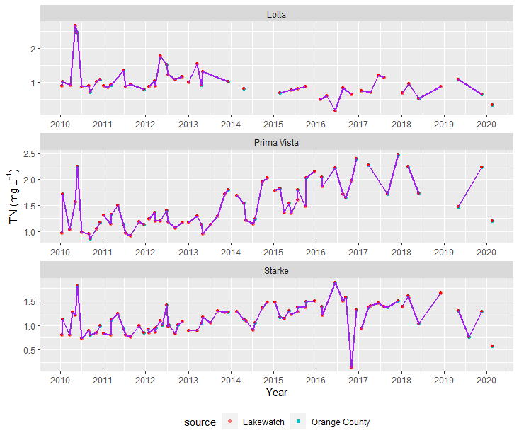
@benjaminhlina So, ran your code and resulted in this plot:
What I am looking for is this:
I made year a factor, but then I could not filter out data after year>2009, as it does not recognize this as a factor.
Any ideas?
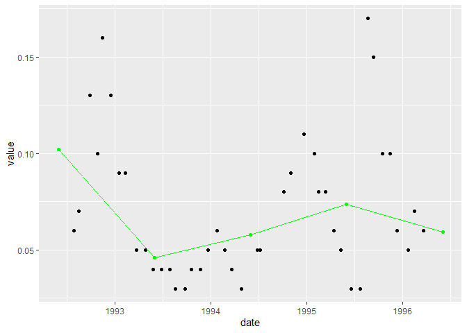
Here is how I would use stat-summary().
library(ggplot2)
library(dplyr, warn.conflicts = FALSE)
library(lubridate)
#>
#> Attaching package: 'lubridate'
#> The following objects are masked from 'package:base':
#>
#>     date, intersect, setdiff, union
tpexample <- tibble::tribble(
  ~lake,     ~source,       ~date, ~parm, ~value,  ~unit,
  "lake1", "lakewatch", "30-Jul-92",  "tp",   0.06, "mg/L",
  "lake1", "lakewatch", "18-Aug-92",  "tp",   0.07, "mg/L",
  "lake1", "lakewatch", "29-Sep-92",  "tp",   0.13, "mg/L",
  "lake1", "lakewatch", "29-Oct-92",  "tp",    0.1, "mg/L",
  "lake1", "lakewatch", "16-Nov-92",  "tp",   0.16, "mg/L",
  "lake1", "lakewatch", "16-Dec-92",  "tp",   0.13, "mg/L",
  "lake1", "lakewatch", "19-Jan-93",  "tp",   0.09, "mg/L",
  "lake1", "lakewatch", "10-Feb-93",  "tp",   0.09, "mg/L",
  "lake1", "lakewatch", "24-Mar-93",  "tp",   0.05, "mg/L",
  "lake1", "lakewatch", "28-Apr-93",  "tp",   0.05, "mg/L",
  "lake1", "lakewatch", "28-May-93",  "tp",   0.04, "mg/L",
  "lake1", "lakewatch", "29-Jun-93",  "tp",   0.04, "mg/L",
  "lake1", "lakewatch", "29-Jul-93",  "tp",   0.04, "mg/L",
  "lake1", "lakewatch", "20-Aug-93",  "tp",   0.03, "mg/L",
  "lake1", "lakewatch", "27-Sep-93",  "tp",   0.03, "mg/L",
  "lake1", "lakewatch", "20-Oct-93",  "tp",   0.04, "mg/L",
  "lake1", "lakewatch", "22-Nov-93",  "tp",   0.04, "mg/L",
  "lake1", "lakewatch", "22-Dec-93",  "tp",   0.05, "mg/L",
  "lake1", "lakewatch", "26-Jan-94",  "tp",   0.06, "mg/L",
  "lake1", "lakewatch", "23-Feb-94",  "tp",   0.05, "mg/L",
  "lake1", "lakewatch", "23-Mar-94",  "tp",   0.04, "mg/L",
  "lake1", "lakewatch", "27-Apr-94",  "tp",   0.03, "mg/L",
  "lake1", "lakewatch", "28-Jun-94",  "tp",   0.05, "mg/L",
  "lake1", "lakewatch",  "9-Jul-94",  "tp",   0.05, "mg/L",
  "lake1", "lakewatch",  "5-Oct-94",  "tp",   0.08, "mg/L",
  "lake1", "lakewatch",  "1-Nov-94",  "tp",   0.09, "mg/L",
  "lake1", "lakewatch", "22-Dec-94",  "tp",   0.11, "mg/L",
  "lake1", "lakewatch", "31-Jan-95",  "tp",    0.1, "mg/L",
  "lake1", "lakewatch", "16-Feb-95",  "tp",   0.08, "mg/L",
  "lake1", "lakewatch", "14-Mar-95",  "tp",   0.08, "mg/L",
  "lake1", "lakewatch", "13-Apr-95",  "tp",   0.06, "mg/L",
  "lake1", "lakewatch", "11-May-95",  "tp",   0.05, "mg/L",
  "lake1", "lakewatch", "20-Jun-95",  "tp",   0.03, "mg/L",
  "lake1", "lakewatch", "25-Jul-95",  "tp",   0.03, "mg/L",
  "lake1", "lakewatch", "21-Aug-95",  "tp",   0.17, "mg/L",
  "lake1", "lakewatch", "12-Sep-95",  "tp",   0.15, "mg/L",
  "lake1", "lakewatch", "16-Oct-95",  "tp",    0.1, "mg/L",
  "lake1", "lakewatch", "14-Nov-95",  "tp",    0.1, "mg/L",
  "lake1", "lakewatch", "12-Dec-95",  "tp",   0.06, "mg/L",
  "lake1", "lakewatch", "23-Jan-96",  "tp",   0.05, "mg/L",
  "lake1", "lakewatch", "15-Feb-96",  "tp",   0.07, "mg/L",
  "lake1", "lakewatch", "20-Mar-96",  "tp",   0.06, "mg/L"
)
tpexample <- tpexample %>% mutate(date = dmy(date),
                                  year = year(date),
                                  MidYear=make_date(year = year,6,1))
ggplot(tpexample,) +
  geom_point(mapping =aes(x=date, y=value,))+
  stat_summary(geom = "point",mapping=aes(x=MidYear,y=value),
               fun = function(z)exp(mean(log(z))),color="green")+
  stat_summary(geom = "line",mapping=aes(x=MidYear,y=value),
               fun = function(z)exp(mean(log(z))),color="green")

Created on 2020-11-21 by the reprex package (v0.3.0)
So from both a stylistic and behind the scene R stand point it's better to make the function outside the ggplot call, than in it. See Hadley's page about stylistic ways to write code and why here. Always break code up into smaller chunks as it's easier for the computer to run, easier to trouble shoot, debug, and read.
gm_mean <- function(x) {
  exp(mean(log(x)))
}
or with pipes which is easier to read but relies on magrittr to be loaded
gm_mean <- function(x) {
  x %>%
    log() %>%
    mean() %>%
    exp()
}
Next as pointed out the one thing I was missing that @FJCC caught is the mid_year column. I've added as such. You should never turn off warning conflicts as this helps you know what other packages have similar functions e.g. dplyr::select(). Select is a common name for many functions in many packages. When you load packages it's helpful to know that information, so you don't run into conlficts. When loading packages it's nice to load them in alphabetical order as it makes it easier to know which ones are loaded and which ones are missing.
# load packages ----
library(dplyr)
library(ggplot2)
library(lubridate)
library(tibble)

# create dataframe  ----
tpexample <- tribble(
  ~lake,     ~source,       ~date, ~parm, ~value,  ~unit,
  "lake1", "lakewatch", "30-Jul-92",  "tp",   0.06, "mg/L",
  "lake1", "lakewatch", "18-Aug-92",  "tp",   0.07, "mg/L",
  "lake1", "lakewatch", "29-Sep-92",  "tp",   0.13, "mg/L",
  "lake1", "lakewatch", "29-Oct-92",  "tp",    0.1, "mg/L",
  "lake1", "lakewatch", "16-Nov-92",  "tp",   0.16, "mg/L",
  "lake1", "lakewatch", "16-Dec-92",  "tp",   0.13, "mg/L",
  "lake1", "lakewatch", "19-Jan-93",  "tp",   0.09, "mg/L",
  "lake1", "lakewatch", "10-Feb-93",  "tp",   0.09, "mg/L",
  "lake1", "lakewatch", "24-Mar-93",  "tp",   0.05, "mg/L",
  "lake1", "lakewatch", "28-Apr-93",  "tp",   0.05, "mg/L",
  "lake1", "lakewatch", "28-May-93",  "tp",   0.04, "mg/L",
  "lake1", "lakewatch", "29-Jun-93",  "tp",   0.04, "mg/L",
  "lake1", "lakewatch", "29-Jul-93",  "tp",   0.04, "mg/L",
  "lake1", "lakewatch", "20-Aug-93",  "tp",   0.03, "mg/L",
  "lake1", "lakewatch", "27-Sep-93",  "tp",   0.03, "mg/L",
  "lake1", "lakewatch", "20-Oct-93",  "tp",   0.04, "mg/L",
  "lake1", "lakewatch", "22-Nov-93",  "tp",   0.04, "mg/L",
  "lake1", "lakewatch", "22-Dec-93",  "tp",   0.05, "mg/L",
  "lake1", "lakewatch", "26-Jan-94",  "tp",   0.06, "mg/L",
  "lake1", "lakewatch", "23-Feb-94",  "tp",   0.05, "mg/L",
  "lake1", "lakewatch", "23-Mar-94",  "tp",   0.04, "mg/L",
  "lake1", "lakewatch", "27-Apr-94",  "tp",   0.03, "mg/L",
  "lake1", "lakewatch", "28-Jun-94",  "tp",   0.05, "mg/L",
  "lake1", "lakewatch",  "9-Jul-94",  "tp",   0.05, "mg/L",
  "lake1", "lakewatch",  "5-Oct-94",  "tp",   0.08, "mg/L",
  "lake1", "lakewatch",  "1-Nov-94",  "tp",   0.09, "mg/L",
  "lake1", "lakewatch", "22-Dec-94",  "tp",   0.11, "mg/L",
  "lake1", "lakewatch", "31-Jan-95",  "tp",    0.1, "mg/L",
  "lake1", "lakewatch", "16-Feb-95",  "tp",   0.08, "mg/L",
  "lake1", "lakewatch", "14-Mar-95",  "tp",   0.08, "mg/L",
  "lake1", "lakewatch", "13-Apr-95",  "tp",   0.06, "mg/L",
  "lake1", "lakewatch", "11-May-95",  "tp",   0.05, "mg/L",
  "lake1", "lakewatch", "20-Jun-95",  "tp",   0.03, "mg/L",
  "lake1", "lakewatch", "25-Jul-95",  "tp",   0.03, "mg/L",
  "lake1", "lakewatch", "21-Aug-95",  "tp",   0.17, "mg/L",
  "lake1", "lakewatch", "12-Sep-95",  "tp",   0.15, "mg/L",
  "lake1", "lakewatch", "16-Oct-95",  "tp",    0.1, "mg/L",
  "lake1", "lakewatch", "14-Nov-95",  "tp",    0.1, "mg/L",
  "lake1", "lakewatch", "12-Dec-95",  "tp",   0.06, "mg/L",
  "lake1", "lakewatch", "23-Jan-96",  "tp",   0.05, "mg/L",
  "lake1", "lakewatch", "15-Feb-96",  "tp",   0.07, "mg/L",
  "lake1", "lakewatch", "20-Mar-96",  "tp",   0.06, "mg/L"
)

# reformat the date column, add in year and add in mid_year column.
# Pipes are meant to be entered afterwards not continued on forwards.

tpexample <- tpexample %>%
  mutate(date = dmy(date),
         year = year(date),
         mid_year = make_date(year = year, 6, 1))

# use glimpse() to assess the structure of the dataframe

glimpse(tpexample)

# plot -----
# I'll be honest, I missed a few things (commas and brackets)
# considering I originally wrote that free hand outside of R in the submission box
# without actually running it on any data.
# I apologize for that. Going forward see fixed plot that works with sample data
# I've commented a few lines as some of that code doesn't run with the reprex data

# group = year was wrong, sorry about that
# but I left it commented as a note so you can see how group works
# facet_wrap is commented as for the reprex data
# there is not ablitiy to facet as such

graph3 <- tpexample %>%
  ggplot() +
  geom_point(aes(x = date, y = value, color = source)) +
  stat_summary(aes(x = mid_year, y = value,
                   # group = year
                   ),
               fun = gm_mean,
               geom = "point",
               size = 1,
               color = "red") +
  stat_summary(aes(x = mid_year, y = value,
                   # group = year
                   ),
               fun = gm_mean,
               geom = "line",
               size = 1,
               color = "purple") +
  # facet_wrap(.~ lake, ncol = 1, scales =  "free",
  #            labeller = labeller(lake = lak.labs)
  #            ) +
  scale_x_date(date_breaks = "1 years", date_labels = "%Y") +
  theme(legend.position = "bottom") +
  labs(x = "Year", y = expression(paste("TP (mg ", L^-1, ")")))

graph3
This produces the same graph whether you put the function inside the ggplot call or not. However, it is always better to do any extra things outside the ggplot call e.g. run and create a function or filter your data. Hope this helps, sorry for not taking a more detailed approach. Again I originally wrote all of that free hand from just looking at was already posted and didn't actually run any of it, that's my mistake, sorry. When making a reprex and updating it make sure that you continue to use the same data or data structure as some of the code doesn't work for the posted reprex data. This makes things difficult when trying to assist.
This topic was automatically closed 21 days after the last reply. New replies are no longer allowed.
If you have a query related to it or one of the replies, start a new topic and refer back with a link.


